Empirical/Graphical, Normal, LogNormal Distributions

Workshop 1, Basic Frequency Analysis

Files needed: workshop 1.xlsx

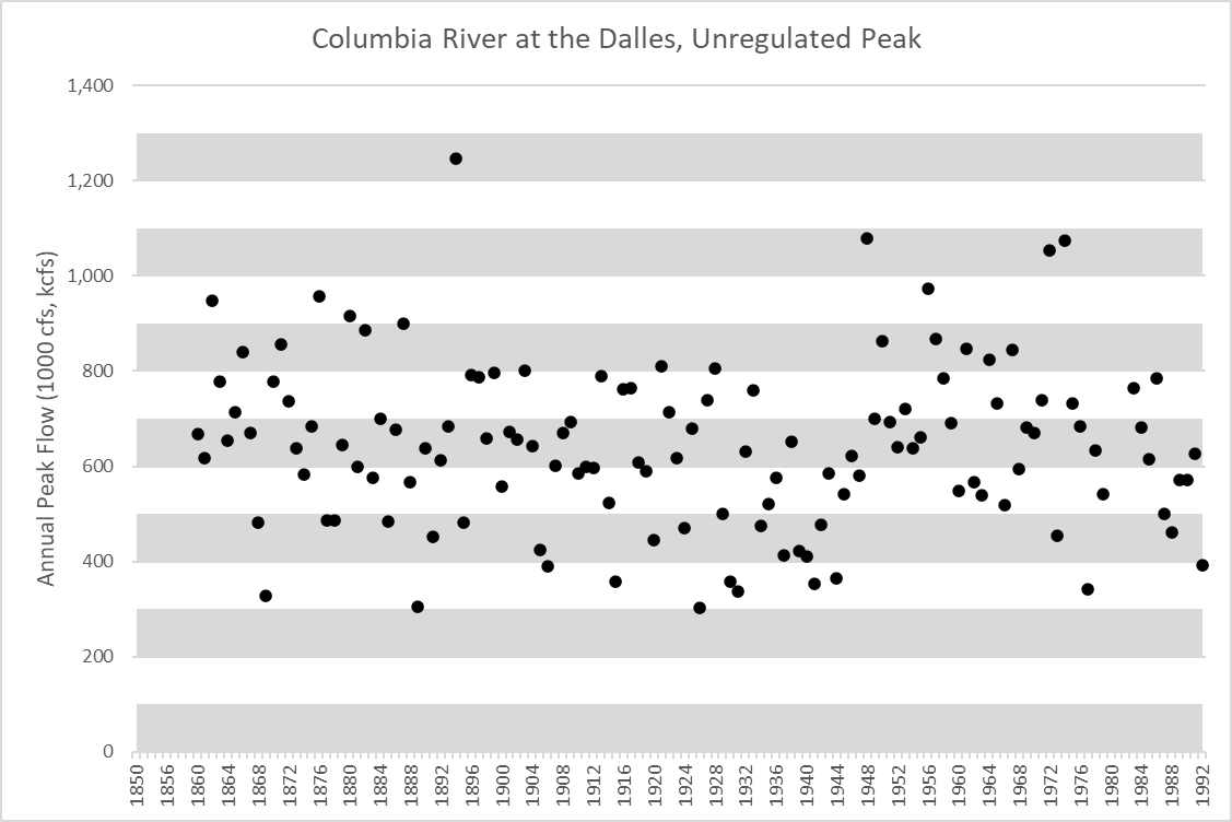
Streamflow records for the Columbia River at the Dalles (USGS Station number 14105700) have been kept since 1858. Since much of the Columbia River Basin is regulated, frequency analysis requires developing a "homogeneous" set of unregulated or natural flows that take reservoir operations into account. The dataset on tab “data” of the spreadsheet “workshop 1.xlsx” lists unregulated (natural) annual peak flows for 135 years of record.

Task 1. Data

Download and open spreadsheet “workshop 1.xlsx.” workshop 1.xlsx
Go to tab “data” and examine the record stored there as table and plots. Note that the flows are first noted in cfs and then in kilo-cfs or kcfs (i.e., 1000-cfs). The top graph is in cfs, and the lower graph is in kcfs, and includes additional color bands. The remainder of this workshop will use kcfs!

Task 2. Graphical Distribution

Go to tab “empirical.”
Create a histogram of the data set, entering counts for 100 kcfs intervals in blue cells G7:G20.
(Cell G7 should contain the the number of values between 0 and 100 kcfs, cell G8 the number between 100 and 200 kcfs, etc.)
There are several way you may proceed, ranging from more simple to more efficient. Use one of the methods below.
1. Count values from the graph. Making use of the gray and white bands on the plot, count the number of values in each 100 kcfs interval. Enter those counts next to the higher value (lower cell) of each interval.
2. Use the countif() function to determine the count in each interval. As an example, in cell G10, enter the following:
```
=COUNTIF($C$5:$C$139,"<"&F7)-COUNTIF($C$5:$C$139,"<"&F6)
```
  This cell equation can be copied to the entire blue range, G7:G20.
3. Use the array function frequency(). Select the blue cells G7:G20, and enter the following the function below.
```
=FREQUENCY(C5:C139,F7:F20)
```
  Note that to finalize an array function, rather than simply hitting Enter, you must hit Control-Shift-Enter at the same time. When finalized in this way, the function will be surrounded by curly brackets, appearing as follows:
  
  {=FREQUENCY(C5:C139,F7:F20)}
  
  With any of these methods, the histogram plots will populate. You’ll find both count and relative frequency histograms, and a cumulative histogram. You’ll also find an empirical CDF which is simply the cumulative histogram plotted as a line, both using the traditional axes, and plotted as a frequency curve.

Task 3. Sample Statistics

Go to tab “statistics” to calculate the mean and standard deviation of your sample.
A table is set up to guide your computation, first calculating the sample mean (or, average) and then the deviations from the mean, and finally summing the squared deviations from the mean and dividing by N-1 to calculate sample variance.
1. Mean, X_bar:
  1. Cell C143 already contains the sum of the flow sample in kcfs, and cell C144 contains the count, N
  2. In cell C145, divide the sum of values by N to compute the sample mean, or average. The entry should look like:
    =C143/C144
  3. In cell C146, use Excel’s average() function for comparison.
2. Deviation from mean, X-X_bar:
  1. Go to the top of the table.
  2. In cell D7, subtract the computed sample mean (in cell C145) from the first sample value of flow in kcfs. Hit the F4 key once to make C145 an absolute reference for both row and column. The entry should look like:
    =C7-$C$145
  3. In Cell E7, square the deviation from the mean. The entry should look like:
    =D7^2
  4. Copy cells D7 and E7 down for the rest of the sample values in rows 8 through 141.
3. Sample Variance, S²:
  1. Cell E143 already contains the sum of the squared deviations from the mean.
  2. In cell E144, compute sample variance by dividing that sum by N-1.
    The entry should look like:
    =E143/(C144-1)
  3. In cell E145, use Excel’s var() function for comparison.
4. Sample Standard Deviation, S:
  1. In cell E146, compute the square root of the variance to compute the standard deviation, S. You can use EITHER
    =sqrt(E144)
    OR
    E144^0.5
  2. In cell E147, use Excel’s stdev() function for comparison.

Task 4. Normal

Assume annual peak discharge follows a Normal distribution.

Go to tab “Normal” in the spreadsheet. Your sample statistics from step (3) should appear at the top of the tab.
You’ll be calculating the Normal distribution CDF in the opposite manner as that shown in the lecture.
The lecture showed specifying cumulative probabilities and computing the flow quantiles as Q_p = X_bar + S * Z_p.
Here, you’ll be specifying flows and computing the probability that the variable is less than each flow.
You'll use the method of converting each flow value to standard Normal variable Z by subtracting the sample mean and then dividing by the standard deviation.
Next, you'll determine the cumulative probability of the standard Normal distribution either by looking up the value on tab “Z table”, or using Excel’s standard Normal approximation.
In cell B12, compute Z by entering
```
=(A12-$C$3)/$C$4
```
Copy cell B12 to the rest of the column of blue cells, in B13:B25
In cell C12, use ONE of the following methods of finding the cumulative probability of your Z values:
1. Look up cumulative probability in Z table.
  1. Note the first value of Z (cell B12) to 2 decimal places.
  2. Go to spreadsheet tab “Z table”. Find the row containing the Z value to 1 decimal place, then go across the columns to find the second decimal value. The value in the resulting cell is the cumulative probability you're looking for.
  3. Type this value in cell C12.
  4. Do the same lookup for the Z values in cells B13:B25.
2. Use Excel’s standard Normal distribution approximation.
  1. In cell C12, enter the standard Normal distribution function as follows:
    =norm.s.dist(B12,true)
    note, “true” refers to the CDF, rather than PDF, and s refers the the standard Normal, rather than Normal
  2. Copy the resulting function down to the rest of the rows, cells C13:C25
Excel also has a function for the Normal distribution that is not the standard Normal found in text book covers.
Using =norm.dist(), you may use the flow value directly as the first argument, rather than transforming it to Z. The mean and standard deviation are entered into the function as the second and third arguments.
1. In cells D12:D25, you'll use Excel’s Normal distribution function for comparison.
2. In cell D12, enter
```
=norm.dist(A12,$C$3,$C$4,true) 
```
3. Copy the cell to the range D13:D25

Note, when columns B and C are filled in as described above, the Normal PDF and CDF will appear on the graphs to the right. The PDF is plotted with the histogram, and the CDF is plotted with the cumulative histogram. To the right, the CDF is also plotted with the data points versus plotting positions using both a linear and log scale for flow.

Task 5. LogNormal Distribution

Assume annual peak discharge follows a logNormal distribution.

Return to tab “statistics.” Note the table in columns J:N repeats the computation of the first table, except using base 10 log of flow.
Repeat the entire step 3 computation of sample mean and standard deviation on log(flow) using this table.
Go to tab “logNormal.” Your sample statistics from the “statistics” tab should appear at the top.
Use those statistics and repeat the instructions of step (4), but on the “logNormal” tab, thus assuming a logNormal distribution.

Task 6. View Plots

Go to the “plots” tab, view the graphs, and consider the three distributions just developed (graphical/empirical, Normal, LogNormal) and how they compare to the plotted data.

Task 7. Compute Probabilities from each Distribution

Go to tab “comps” to answer the following questions from each curve: (more guidance below)
1. The probability of observing a peak flow (Q) between 700,000 and 800,000 cfs,
  i.e., P(700,000 ≤ Q ≤ 800,000).
2. P(Q ≤ 450,000)
3. P(Q ≥ 10⁶)
4. The peak discharge which has a 1% chance of being exceeded in any given year; a 50% chance.

The cells on the left portion of the tab can refer back to the the previous tabs to answer when the result has already been computed there. Where needing results not previously computed, try using the functions =normdist() and =norminv(), which are Normal distributions that are NOT standard normal, and thus include mean and standard deviation as arguments, as in step 6 of Task 4.

On the right side of the tab, values for Normal and LogNormal are computed using standard Normal, as on the previous tabs.

Note, tab "comps done" holds the results. The bold purple cells answer each question in the most efficient way, given Excel tools, in columns F, H and J. In columns M thorough S, the values are computed in the more traditional way. Review the computations shown.

The solution to this workshop is in file "workshop 1 SOLUTION.xlsx" workshop 1 SOLUTION.xlsx