Download PDF
Download page Task 3. Annualize Partial Duration Series and Compare with Annual Maximum Series.
Task 3. Annualize Partial Duration Series and Compare with Annual Maximum Series
The following annualization methods will be used in this task. Annualization is the conversion of exceedance probabilities from partial duration space to annual exceedance probabilities.
The implementation of these equations has been performed for you in the provided spreadsheet.
Empirical: Langbein (1949)
The relationship between empirical flood expectancies in the partial duration series and the probability of the corresponding flood as an annual series is given by (Langbein, 1949):
p = exp[-\lambda * (1 - p_P_D_S)]
where p is annual non-exceedance probability, pPDS is the partial duration non-exceendace probability, and \lambda is the rate of flood events (\lambda = m/N where m is the number of events in the partial duration series and N is the number of years).
Analytical: Madsen et al. (1997)
The relationships between the Generalized Pareto distribution parameters location \xi, scale \alpha, and shape \kappa and Generalized Extreme Value distribution parameters location \xi *, scale \alpha *, and shape \kappa * are (Madsen et al., 1997):
\xi* = \xi + \frac {\alpha}{\kappa} (1 - \lambda ^ - ^ \kappa)
\alpha * = \alpha \lambda ^ - ^ \kappa
\kappa * = \kappa
References:
Langbein, W. B. (1949). Annual Floods and the Partial-duration Flood Series. American Geophysical Union, 30(6), 879-881.
Madsen, H., Rasmussen, P., and Rosbjerg, D. (1997). Comparison of annual maximum series and partial duration series methods for modeling extreme hydrologic events 1. At-site modeling. Water Resources Research, 33(4), 747-757.
- Open the Excel spreadsheet provided at the beginning of this workshop (Partial Duration Series using HEC-SSP and Excel). The spreadsheet contains 7 tabs:
- AMS - Empirical
- AMS - Analytical (GEV)
- Empirical (Langbein)
- Analytical (Madsen)
- Curves
- Frequency Chart
- Chart Setup
- In the following steps, you will enter values in the first four tabs to populate the Curves and Frequency Chart tab. You will not need to modify the Chart Setup tab.
- Navigate to the tab named AMS - Empirical.
- Copy and paste the annual maximum series events from HEC-SSP into the orange cells in column A.
- Right click on the AMS data set in HEC-SSP and select Tabulate.
- Hold the Ctrl button and select all flow values in the right-most column.
- Right click and select Copy. Navigate back to Excel and paste into column A.
- Enter 89 in cell B2 as the number of years.

- Sort the flow values from latest to smallest so that the largest flow value is in cell A6.
- Highlight all flow values.
- Select the Data tab.
- Within the Sort & Filter group, select the Sort Largest to Smallest button
 .
. - If you are prompted with a Sort Warning, select the Continue with the current selection option to only sort the column A values (shown below).

- Navigate to the tab named AMS - Analytical (GEV).
- Copy and paste the frequency curve ordinates from HEC-SSP's Distribution Fitting Analysis.
- Open the Distribution Fitting Analysis named AppleRiver_AMS.
- Navigate to the Results tab.
- Copy the Median Curve column in the Frequency Curves panel (boxed in red below).

- Paste the values in the orange cells in column B of the AMS - Analytical (GEV) tab in Excel.
- Navigate to the tab named Empirical (Langbein).
- Copy and paste the PDS5 events from HEC-SSP into the orange cells in column A.
- Right click on the PDS5 data set in HEC-SSP and select Tabulate.
- Hold the Ctrl button and select all flow values in the right-most column.
- Right click and select Copy.
- Navigate back to the Empirical (Langbein) tab Excel and paste the values into column A.
- Enter the number of PDS events in cell B2.
- Enter 89 in cell B3 as the number of years.
 Tab")
- The rate parameter in cell B4 should be auto-populated.
- Sort the flow values from largest to smallest so that the largest flow value is in cell A8.
- The probabilities in columns C-E will be computed based on the values in cells B2:B4.
- Navigate to the tab named Analytical (Madsen).
- Open the Distribution Fitting Analysis named AppleRiver_PDS5.
- Navigate to the Results tab.
- Copy the Generalized Pareto distribution parameters from the Distribution Parameters panel into the orange cells in the Excel sheet. Also, enter the number of PDS events and years.

 Tab")
- The parameters of the Generalized Extreme Value distribution (location, scale, and shape) are computed for you in cells B9:B11. Click within these cells to view the equations. Notice that these equations are the same as those provided within the green box at the top of this page.
- The frequency curve ordinates in cells B15:B25 will be computed for you.
- Navigate to the Curves tab. Notice that there are 4 frequency curves:
- The empirical annualization of the PDS events
- The analytical annualization of the Generalized Pareto distribution, fit to the PDS, using the conversion between the Generalized Pareto distribution to the Generalized Extreme Value distribution
- The empirical probabilities of the AMS
- The GEV distribution frequency curve ordinates, fit to the AMS events
- Navigate to the Frequency Chart tab and examine the results. Note that the analytical frequency curves are plotted as lines in Excel but because we only computed 12 frequency ordinates, they may not look smooth.
QUESTION 5: Why did we not use the PDS plotting positions, column C in the Empirical (Langbein) tab, when plotting the frequency curve?
The PDS plotting positions do not represent annual exceedance probability (AEP) since the number of events in the PDS is not equivalent to the number of years of record. In order to make an apples-to-apples comparison with an annual maximum series frequency curve or plotting positions, the PDS plotting positions must be annualized.
QUESTION 6: Do the empirical and analytical results align? First, turn off the empirical curves and look at just the analytical curves. Then turn off the analytical curves and look at the empirical curves.
In this case, the four frequency curves plot nearly on top of each other. This is not always the case when comparing a frequency curve computed from a PDS to one computed from an AMS!
The two analytical curves exhibit slight differences at the tails. The two empirical curves are nearly identical for probabilities less frequent than 0.8 but diverge for probabilities more frequent than 0.8.


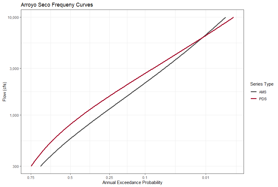
In arid regions, using an annual maximum series approach may omit large flood events. A stream in an arid region might experience multiple floods in one year and no floods in the next few years. As a result, the annual maximum series "throws away" the 2nd, 3rd, etc. largest floods in a year while the partial duration series would include those floods, as long as they exceed a sufficiently high threshold. The figure below shows the empirical and analytical frequency curves from a PDS (pink) and AMS (grey) at Arroyo Seco near Pasadena, CA (USGS 11098000). The AMS omits 2 of the top 6 floods at the site and that the frequency curve derived from the PDS plots higher than the AMS curve for annual exceedance probabilities up to ~ 0.01 (1/100).
This workshop used mean daily streamflow data. In flood frequency analysis, instantaneous data is typically used to ascertain frequency-based peak flow estimates. However, instantaneous streamflow records are typically much shorter than mean daily streamflow records. In addition, conversion of mean daily streamflow to instantaneous streamflow is possible but introduces uncertainty to the frequency curve.
Extra Time?
Select a different partial duration series (PDS1, PDS2, PDS3, PDS4, or PDS6) and repeat Tasks 2 and 3. Re-visit question 6 with your new annualized partial duration series.