Introduction

In this workshop you will work with a spreadsheet containing the results of a number of virtual dice rolls. You will be asked to estimate some properties of the population of dice rolls from summaries of the data that were gathered, and also to fit models to the data.

Each result was generated by rolling 3 6-sided dice and taking the sum of the rolls. For example, if the 3 dice turned up $\begin{array}{l}[3,6,4]\end{array}$ , the result would be 13. The rolls were pasted in the Outcome column of the data so that they don't change, but if you want to generate your own rolls in this manner, you can see how below.

In Excel, the RANDBETWEEN() function returns a random integer between two endpoints, inclusive of the endpoints. To generate a single six-sided die roll, RANDBETWEEN(1,6) is used. To generate the rolls in this sample data, add together three rolls like this: RANDBETWEEN(1,6)+RANDBETWEEN(1,6)+RANDBETWEEN(1,6). You can't use 3 * RANDBETWEEN(1,6) because that would generate one random die roll and then multiply it by 3, instead of taking the sum of 3 independent dice rolls.

The Excel workbook needed to start the workshop is here: Probability WS Start.xlsm

Workshop

Sample Statistics

Start on the "100 Rolls" worksheet of the Excel workbook. On the left side there are two columns of data in columns A and B: an index column containing the roll number, and a column of the totals of the dice rolls. There is also a count histogram table in columns E and F of the worksheet.

Question 1: What kind of random variable is this? What is its support?

The rolls can only take on integer values, and they are on a closed interval. This is a discrete random variable. It has support on the integers, with a closed interval of $\begin{array}{l}[3,18]\end{array}$ .

The count of each of the possible outcomes is shown in column F.

Question 2: What is the sample mode?

The outcome of 11 has a count of 13 which is more than any other outcome, making it the most frequent outcome and therefore the sample mode.

An empty table of sample statistics is below the count histogram. Fill in the sample mode based on what you see in the count histogram.

Fill in the sample minimum and sample maximum using the Excel MIN() and MAX() functions on the array of data in column B.

In the count histogram table, the outcome of 3 has a count of zero. We know that a roll of 3 is possible.

Question 3: Considering physical probability, what is the probability of rolling a 3 as the total of 3 fair dice? Do you think seeing zero 3s in 100 rolls is unusual?

There is only one way to roll a 3, by rolling a 1 on each die. The probability of rolling a 1 on a fair die is $\begin{array}{l}\frac{1}{6}\end{array}$ due to physical probability. Because the rolls are independent, the joint probability of rolling a 1 on three separate dice is $\begin{array}{l}\frac{1}{6}*\frac{1}{6}*\frac{1}{6}=\frac{1}{216}\approx0.00463\end{array}$ . This is a fairly rare event, occurring on average once in 216 rolls. It wouldn't be too unusual to miss out on seeing one in 100 rolls.

Fill in the sample median and sample mean. Excel has the functions MEDIAN() and AVERAGE() to compute these for you.

Question 4: What kind of sample statistics are the mode, median, and mean? What are their values for this dataset? What does that seem to imply about the shape of the data? What sample statistic would you use to confirm this?

Mode, median, and mean are measures of central tendency. The mode and median are both 11, and the mean is 10.89 which is close to 11. Since all the measures of central tendency are close together, it seems to imply the dataset is symmetrical. You could use the coefficient of skewness to check if the dataset is symmetrical. If it is, the skew will be close to 0.

Fill in the sample variance and the sample standard deviation. Make sure to use the Excel functions VAR.S() and STDEV.S() to compute the sample statistics.

Question 5: What is the relationship between the variance and standard deviation?

The standard deviation is the square root of the variance.

Finally, add in the sample coefficient of skewness using the function SKEW().

Question 6: Based on information you've gathered previously, is the value you see for sample skew expected or unexpected?

Hopefully you won't be too surprised to see that the value of skew (-0.07) is close to zero, since you saw that the mode, median, and mean, are all close together. In total these measures seem to imply the data show some symmetry.

Let's say that we're most interested in knowing how often outcomes greater than 11 occur. Below the sample statistics table is an entry for "Empirical $\begin{array}{l}p(X > 11)\end{array}$ ."

Question 7: What outcomes are included in the event $\begin{array}{l}X>11\end{array}$ ? How would you estimate the relative frequency of this event? What is the relative frequency of $\begin{array}{l}X>11\end{array}$ ?

The rolls greater than 11 are 12, 13, 14, 15, 16, 17, and 18. To compute the relative frequency of $\begin{array}{l}X>11\end{array}$ you can compute the total number of times those outcomes happen and divide them by the total number of rolls. The total number of results greater than 11 is 44, and there were 100 rolls, so the relative frequency of $\begin{array}{l}X>11\end{array}$ is 0.44.

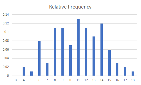
Next, add a new column next to the count histogram labeled "Relative Frequency." Compute the relative frequency for each of the outcomes.

Question 8: What is the sum of the relative frequencies?

The sum of the relative frequencies should be 1, since the probability of the sample space (all the things that can happen) is 1.

Next to the column for the relative frequencies, add a column for "Cumulative Relative Frequency." This column will compute the relative frequency of rolls less than or equal to the outcome in the row of the table. Compute the cumulative relative frequency for each outcome.

Question 9: What is the relative frequency for $\begin{array}{l}X\leq11\end{array}$ ? What does this mean the relative frequency for $\begin{array}{l}X>11\end{array}$ must be? What is the relative frequency for $\begin{array}{l}X\leq18\end{array}$ ?

The relative frequency for $\begin{array}{l}X\leq11\end{array}$ is 0.56. To compute the relative frequency for $\begin{array}{l}X>11\end{array}$ from this value, use the complement, $\begin{array}{l}1-p(X\leq11) = p(X>11) = 1-0.56=0.44\end{array}$ . The relative frequency for $\begin{array}{l}X\leq18\end{array}$ is 1, because all possible outcomes are less than or equal to 18.

Create a plot of your relative frequency histogram and your empirical cumulative distribution function.

First, create a new bar chart by going to the Insert menu in the Excel ribbon, and selecting the Column Charts, Clustered Column like in the screenshot below.

Right click on the new chart and pick "Select Data..." First add a new series by pressing the Add button under Legend Entries (Series) and in the window that pops up (Edit Series) type in for a name "Relative Frequency" and then for series values, select the upward arrow icon. Then, highlight the Relative Frequency column of your table and hit Enter. After the series values are filled in, select OK. Next, edit the Horizontal (Category) Axis Labels by selecting the Edit button, hitting the arrow button in the Axis Labels box that pops up, and then selecting the values in the Outcome column of your table. Hit enter after selecting them, then OK, and then OK one more time to exit the data source selection. The resulting chart should look like this:

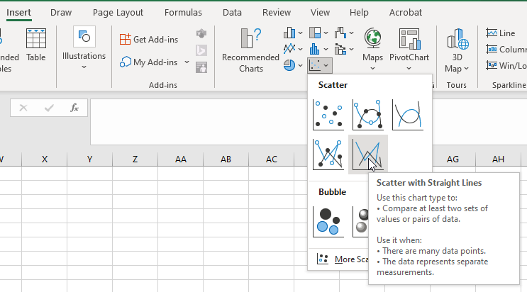
Next, create an empirical CDF. Start by creating a new Scatter with Straight Lines plot by going to the Insert menu, then Insert Scatter (X, Y) or Bubble Chart, then Scatter with Straight Lines like in the screenshot below.

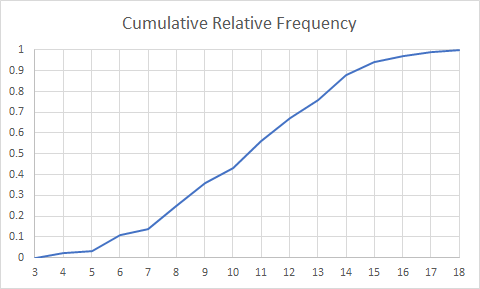
Right click on the new chart and pick "Select Data..." and then add a new series using the Add button. For Series name call it "Cumulative Relative Frequency." Pick the Outcomes column of your table as the X values, and the Cumulative Relative Frequency as your Y values. Once you've entered the data, the chart should look like this:

Adjust the plot extents so they make more sense by right-clicking first on the Y-axis and selecting Format Axis... Change the maximum to be 1. Next right-click on the X-axis and select Format Axis... and set the minimum to 3 and maximum to 18. Change the Major Units to 1. The chart should look like this.

Population Models

You will fit two models to your sample data in order to estimate the population probability distribution. The two models are the triangular distribution and the normal distribution. Note that these distributions are for continuous random variables. Since we we have a relatively large number of outcomes, we can approximate the outcomes with a continuous distribution. It would be less feasible to model a discrete random variable with a continuous distribution if there were fewer outcomes. Remember that the PDF of these distributions doesn't represent the probability of each outcome - although their magnitudes could be close to the sample's relative frequency magnitudes/values! We can only compare probabilities for continuous distributions or variables using intervals or ranges.

Triangular Distribution

The triangular distribution is a 3-parameter probability distribution that is useful for building a simple probability model for a population. Its name comes from the shape of the probability density function, which forms a triangle. Note that it is a continuous probability distribution, and we are treating our discrete data as continuous for this modeling.

Question 10: Looking at the Wikipedia article for the triangular distribution linked above (or recalling the lecture), what do each of the three probability distribution parameters represent?

The three parameters are a, b, and c; a is the lower endpoint of the distribution, b is the upper endpoint of the distribution, and c is the mode of the distribution.

Question 11: What sample statistics would you use to estimate the population probability distribution parameters for the triangular distribution? Hint: we have estimated these already.

For a, which is the distribution's minimum, you would use the sample minimum. For b, which is the distribution's maximum, you would use the sample maximum. And for c, which is the distribution's mode, you would use the sample mode.

The triangular distribution isn't in Excel, but the workbook you have been provided has a custom function for computing its PDF and CDF.

Add two new columns to your table: "Triangular PDF" and "Triangular CDF".

Compute the triangular distribution PDF using the TRIANG_DIST() function. The function requires five arguments in this order:

Argument	Description
x	Value to evaluate the function at
a	Lower bound of the distribution
b	Upper bound of the distribution
c	Mode of the distribution
cumulative	If TRUE, the function returns the cumulative distribution function, if FALSE, the function returns the probability density function.

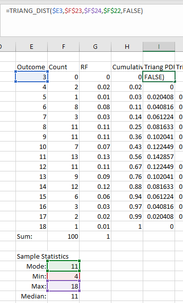
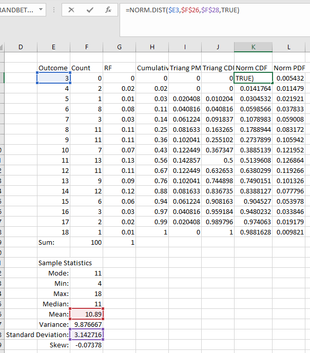
For x, make sure the outcome is set to the first value in the column with your outcomes. For a, set the lower bound to the sample minimum value. For b, set the value to the sample maximum value. For c, set the value to the sample mode. Then, set cumulative to FALSE so it computes the probability density function. TIP: when you set the function values for a, b, and c, lock the cell references to the cells that contain the sample values using the F4 key. An example is shown below.

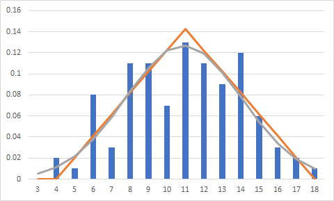
Add the new PDF to your histogram by right-clicking on the chart and picking Select Data... and then add a new series called Triangular Distribution. Choose the PDF values you just computed as the series values. After adding that series, right click on the chart and select "Change Chart Type." Go to the bottom and select "Combo" and then set the chart type for the Triangular Distribution to "Line" (if that's selected by default just hit OK.)

Question 12: How well does the triangular distribution represent our sample's shape based on the histogram plots? What potential issues arise with using this distribution for this sample? What would be a way to fix this issue?

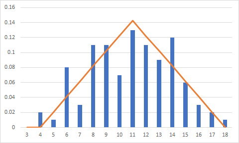
The triangular distribution seems to be more peaked than our data - there seems to be a lot of equal probability in outcomes between 8 and 14 in our data but the triangular distribution has much more of a point at our data mode (11). It doesn't seem to be a great fit from this view. Also, the distribution assigns zero probability density to the outcome of 4 despite us having 2 outcomes of 4 in our sample. This is because the triangular distribution doesn't give any probability to the outcomes right at the endpoint. We could adjust our endpoint down to 3 (which is the true lower bound of our data) which would allow there to be probability mass at 4.

Histogram and PDF with lower bound at 4 (sample minimum):

Histogram and PDF with lower bound of triangular distribution ("a" parameter) set manually to 3:

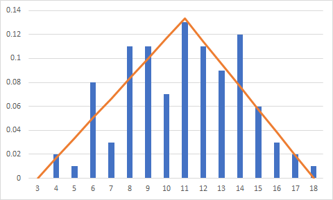
The result looks better, but there is still a lot of variability in our dataset in comparison with this distribution.

Fill in the "Triangular CDF" column using the TRIANG_DIST() function. For x, make sure the outcome is set to the first value in the column with your outcomes. For a, set the lower bound to the sample minimum value. For b, set the value to the sample maximum value. For c, set the value to the sample mode. Then, set cumulative to TRUE so it computes the cumulative distribution function. TIP: when you set the function values for a, b, and c, lock the cell references to the cells that contain the sample values using the F4 key. An example is shown below.

Next, add the triangular CDF to the empirical CDF plot. Right click on the plot and select Select Data... then add a new series. Call it "Triangular Distribution" and set the X-values to the outcomes, and the Y values to the triangular distribution CDF values.

Question 13: How well does the triangular distribution represent our sample based on the CDF plots? What potential issues arise with using this distribution for this sample? What would be a way to fix this issue?

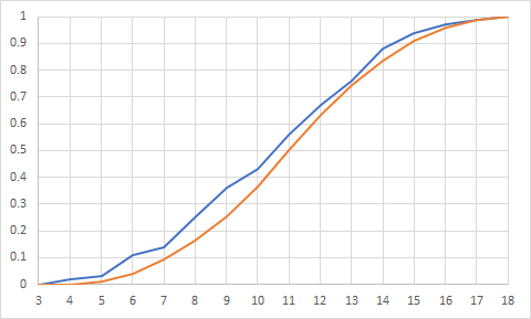
The triangular CDF is below the empirical CDF for the whole range of values. Mainly this is because the CDF at the sample minimum (4) is equal to zero, when our empirical CDF is 0.02. One issue is that the triangular distribution does not give any probability to the values at the endpoints! The other is that because we set the endpoints from the sample minimum and maximum using this distribution, we can't estimate any outcomes outside of that range (for example a roll of 3 which is possible but did not occur in our sample.) We could adjust the value of the "a" parameter to be 3 to make sure our distribution includes the full range of possible outcomes.

Here are the CDFs without adjusting the "a" parameter (blue is empirical, orange is triangular):

Here they are after adjusting the "a" parameter from 4 to 3, again with the empirical in blue and the triangular in orange:

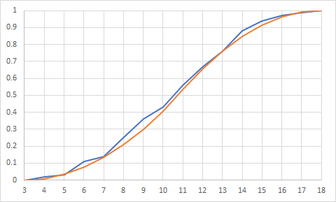
Notice how much better the distribution fit seems to be when getting that endpoint correct!

Normal Distribution

The normal distribution is a 2-parameter probability distribution that is the most commonly-encountered probability distribution in statistics. Note that it is a continuous probability distribution, but we will use it to model a discrete random variable. It produces a probability density function with the familiar bell-curve shape.

Question 14: Looking at the Wikipedia article for the normal distribution linked above (or recalling the lecture), what do each of the two probability distribution parameters represent? What sample statistics would you use to estimate the population probability distribution parameters? Hint: we have estimated these sample statistics already.

The normal distribution is parameterized by its mean $\begin{array}{l}\mu\end{array}$ and its standard deviation $\begin{array}{l}\sigma\end{array}$ . It would be easiest to estimate these with the sample mean and sample standard deviation, respectively.

Question 15: What is the support of the normal distribution? What does that mean with regard to our dataset, in terms of the values the distribution can take on vs. the ones our sample has?

The normal distribution can take on any real number, from negative infinity to infinity. Our dataset can only take on the integers 3 through 18. That means using the normal distribution as a model for our values will have some probability for values less than 3 or greater than 18 which we know aren't possible. So, we need to be careful in interpreting what the model gives us.

Add two new columns to your table: "Normal PDF" and "Normal CDF".

Compute the normal distribution PDF using the NORM.DIST() function. The function requires four arguments in this order:

Argument	Description
x	Value to evaluate the function at
mean	Mean of the population distribution
standard_dev	Standard deviation of the population distribution
cumulative	If TRUE, the function returns the cumulative distribution function, if FALSE, the function returns the probability density function.

For x, make sure the outcome is set to the first value in the column with your outcomes. For mean, set the distribution mean to the sample mean value. For standard_dev, set the value to the sample standard deviation value. Then, set cumulative to FALSE so it computes the probability density function. TIP: when you set the function values for the mean and standard deviation, lock the cell references to the cells that contain the sample values using the F4 key. An example is shown below.

Add the new PDF to your histogram by right-clicking on the chart and picking Select Data... and then add a new series called Normal Distribution. Choose the PDF values you just computed as the series values. After adding that series, right click on the chart and select "Change Chart Type." Go to the bottom and select "Combo" and then set the chart type for the Normal Distribution to "Line" (if that's selected by default just hit OK.)

Question 16: How well does the normal distribution represent our sample's shape based on the histogram plots? What potential issues arise with using this distribution for this sample? What would be a way to fix this issue?

The normal distribution seems fairly reasonable - it is not as peaked as the triangular distribution and provides some probability to the data at the endpoints. It even provides an estimate for the outcome of 3, which we know is possible but we didn't see in our sample. The normal distribution like any other continuous distribution provides non-zero probability density to values in-between our possible values, such as 3.5. The problem is that the probability of rolling a 3.5 or less is the same as the probability of rolling a 3 - because until you get to 4 the probability doesn't increase. The normal distribution doesn't know this, and smoothly accumulates probability between those values. A major problem is that the normal distribution also provides estimates of probability for outcomes like 2 and 19, which are not possible, but the distribution is unbounded so it could even go off to values like -100 or 99999 albeit with tiny probability. The triangular is below in orange, and the normal in grey.

The fix is kind of a bonus answer - you could restrict the domain of the normal distribution by means of a truncated probability distribution. You adjust the PDF of the distribution and increase it by dividing by the amount of probability between the two endpoints you choose, so that the resulting PDF after division still has an area of 1 underneath it.

Fill in the "Normal CDF" column using the NORM.DIST() function. For x, make sure the outcome is set to the first value in the column with your outcomes. For mean, set the distribution mean to the sample mean value. For standard_dev, set the value to the sample standard deviation value. Then, set cumulative to TRUE so it computes the cumulative distribution function. TIP: when you set the function values for the mean and standard deviation, lock the cell references to the cells that contain the sample values using the F4 key. An example is shown below.

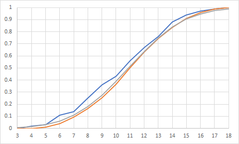
Next, add the normal CDF to the empirical CDF plot. Right click on the plot and select Select Data... then add a new series. Call it "Normal Distribution" and set the X-values to the outcomes, and the Y values to the normal distribution CDF values.

Question 17: How well does the normal distribution represent our sample based on the CDF plots?

The normal distribution doesn't look terribly different than the triangular distribution on this plot and generally under-predicts the cumulative probability when comparing it to the cumulative relative frequency. The triangular is shown in red and the normal in grey.

Question 18: Using the triangular and normal distributions, what is the probability of an outcome greater than 11? What is one problem with computing this value using these distributions?

For the triangular distribution, use the formula 1-TRIANG_DIST(11, a, b, c, TRUE) and for the normal distribution, use the formula 1-NORM.DIST(11, mean, std_deviation, TRUE). For the triangular distribution this value is 0.5, because the distribution is symmetrical (the average of the endpoints, 4 and 18, is equal to the mode, 11). For the normal distribution this value is 0.486. The problem of treating a discrete random variable as continuous happens again - the results are affected by the probability density that each distribution assigns to outcomes between 11 and 12, which aren't possible in our actual dice roll. Care definitely needs to be taken in using continuous distributions for discrete data.

Solution File

A spreadsheet showing the results of the workshop is available here: Probability WS Solution.xlsm

Download PDF

Probability and Statistics Foundations Workshop