Numerical Integration

Background

There are multiple ways to solve the integrals in the expected moments equation.

$//<![CDATA[ \begin{array}{l}E\left[(X-M)^{n}\right]=\frac{\int_{X_{l}}^{X_{u}}(x-M)^{n} f(x) d x}{\int_{X_{l}}^{X_{u}} f(x) d x}\end{array} //]]>$

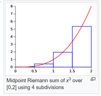
Analytical methods can provide an exact answer and numerical methods can provide an approximate answer. The numerical method used in this study guide is called a midpoint Riemann sum. This is also known as the midpoint rule or rectangle rule and is displayed within Figure 1. This is not the method used in HEC-SSP. However, the Riemann sum method demonstrates the concepts in a way that is more practical and intuitive for civil engineers.

https://en.wikipedia.org/wiki/Numerical_integration

https://en.wikipedia.org/wiki/Riemann_sum

The expected moments equation is a weighted average calculation. An expected moment is an estimate of the nth moment averaged over all the possible flow values within the flow interval.

$//<![CDATA[ \begin{array}{l}E\left[(X-M)^{n}\right]=\frac{\int_{X_{l}}^{X_{u}}(x-M)^{n} f(x) d x}{\int_{X_{l}}^{X_{u}} f(x) d x}\end{array} //]]>$

In numerical integration, the continuous distribution (or frequency curve) defined by f(x) is replaced by a discrete step function defined by a set of rectangles. When this is done, the integrals (∫) in the expected moments equation can be replaced with sums (∑) and calculated as a weighted average.

The general equation for a weighted average is shown below.

$//<![CDATA[ \begin{array}{l}\bar{y}=\frac{\sum_{i=1}^{p} w_{i} y_{i}}{\sum_{i=1}^{p} w_{i}}\end{array} //]]>$

Substituting  = E(X-M)ⁿ, w = f(x)*dx, and y=(X-M) ⁿ gives the midpoint Riemann sum approximation for the nth expected moment where p is the number of rectangles.

$//<![CDATA[ \begin{array}{l}E\left[(X-M)^{n}\right]=\frac{\sum_{i=1}^{p} f(x i) * d x i * E\left(x_{i}-M\right)^{n}}{\sum_{i=1}^{p} f(x i) * d x i}\end{array} //]]>$

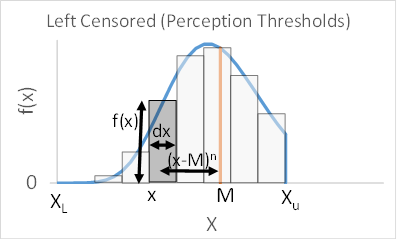
Figure 2 depicts the calculation of an expected moment for a perception threshold using the midpoint Riemann sum method. The calculations are similar for a flow interval. The calculation is performed for values of X=Log(Q) between the low value (X_L) and the high value (X_U) that define the flow interval. In the numerator of the expected moments equation, the height of each rectangle is equal to f(xi) which is the probability density for the LP3 distribution at a flow equal to xi. The width of each rectangle is equal to dxi. The area of each rectangle is equal to f(xi) * dxi. This area is the probability (or weight) given to each rectangle in the weighted average calculation. This weight is analogous to the mass of an object when calculating moments in engineering mechanics. The distance between the mean (M) of the LP3 frequency curve and the value of xi is equal to Xi-M. This distance defines the central moment using the mean of the LP3 distribution as the fixed reference point. The distance is raised to the nth power for the nth moment. This is the definition of a moment. The expected moments equations are calculating the weighted average of this distance raised to the n power over all the possible values of X in the flow interval. In the denominator of the expected moments equation, the total probability (or total weight) is equal to the total area of the rectangles which is an estimate of the area under f(x) between X_L and X_U. This is equal to the total probability for all the possible flow values in the flow interval.

Exercise

Estimate expected moments for flow intervals and perception thresholds

The second step in EMA is to estimate the expected moments for the flow intervals and the perception thresholds based on the parameter estimates from the previous iteration. This exercise uses the midpoint Riemann sum method with twenty rectangles.

$//<![CDATA[ \begin{array}{l}E(X-M)^{n}=\frac{\sum_{i=1}^{p} f(x i) * d x i * E(X-M)^{n}}{\sum_{i=1}^{p} f(x i) * d x i}\end{array} //]]>$

Question 16. Use the “EMA Iteration 1 – Step 2” worksheet in the EMA_Exercise_ManualCalculations v2.0.0.xlsb workbook to calculate the expected moments. The formulas for the flow interval have already been entered. Using these calculations as a guide, calculate the expected moments for the perception threshold.

Note: The low flow value for a flow interval defined by a perception threshold is technically zero (or tau when skew is positive). This causes a problem in the manual calculations because Log(Q) is undefined when Q=0. This exercise avoids the problem by calculating a low flow value (X_L) at an AEP very close to 1. The AEP assumed in this exercise is AEP=0.999999999 or F(x) = 1E-9. This can be seen in cell C46 on the “EMA Iteration 1 – Step 2” worksheet. This method ensures that Q is positive and Log(Q) can be calculated for each EMA iteration. Using an AEP very close to 1 ensures that only a tiny portion of f(x) is excluded from the calculations which should result in a negligible error. This is not the only way to solve this problem.

The third step in EMA is to update the estimates for mean, standard deviation, and skew using the exact (systematic) data and the expected moments for the censored data from the previous exercise. The equations for mean, standard deviation, and skew are provided below. In these equations, X are the exact flow values, E(X) and E(X-M) are the expected moments for the censored data, N_s is the total number of exact flow values, N_C is the total number of censored flow values, M_k is the mean estimate from the current EMA iteration (EMA Iteration 1 – Step 3), M_k-1 is the mean estimate from the previous EMA iteration (EMA Iteration 0 – Step 1), S_k is the standard deviation estimate from the current EMA iteration (EMA Iteration 1 – Step 3), and S_k-1 is the standard deviation estimate from the previous EMA iteration (EMA Iteration 0 – Step 1).

$//<![CDATA[ \begin{array}{l}M_{k}=\frac{\sum_{i=1}^{N_{s}} X_{i}+\sum_{j=1}^{N_{c}} E\left[X_{j}\right]}{N_{s}+N_{c}}\end{array} //]]>$

$//<![CDATA[ \begin{array}{l}S_{k}=\sqrt{\frac{\frac{N_{s}}{N_{s}-1} \sum_{i=1}^{N_{s}}\left(X_{i}-M_{k}\right)^{2}+\sum_{j=1}^{N_{c}} E\left(X_{j}-M_{k-1}\right)^{2}}{N_{s}+N_{c}}}\end{array} //]]>$

$//<![CDATA[ \begin{array}{l}G_{k}=\frac{\frac{\frac{N_{s}{ }^{2}}{\left(N_{s}-1\right)\left(N_{s}-2\right)} \sum_{i=1}^{N_{k}}\left(X_{i}-M_{k}\right)^{3}}{S_{k}^{3}}+\frac{\sum_{j=1}^{N_{c}} E\left(X_{j}-M_{k-1}\right)^{3}}{S_{k-1}^{3}}}{\left(N_{S}+N_{c}\right)}\end{array} //]]>$

Question 17. Using the “EMA Iteration 1 - Step 3” worksheet, estimate the LP3 parameters (mean, standard deviation, and skew) using both the systematic flow values and the expected moments for the historic flow and perception threshold.

Repeat previous steps until convergence

The final step in EMA is to repeat Steps 2 and 3 until the parameter estimates converge. Create a copy of the “EMA Iteration 1 – Step 2” and “EMA Iteration 1 – Step 3” worksheets. Rename the copied worksheets to “EMA Iteration 2 – Step 2” and EMA Iteration 2 – Step 3”.

Question 18. Calculate the expected moments and parameter estimates for the 2^nd EMA iteration. Use the parameter estimates from EMA Iteration 1 – Step 3 to calculate the expected moments in EMA Iteration 2 – Step 2. Use the expected moments from EMA Iteration 2 – Step 2 to calculate the parameter estimates in EMA Iteration 2 – Step 3.  Repeat this process for the 3^rd, 4^th, and 5^th EMA iterations.  Report the results for the 5^th EMA iteration to three decimal places.

Question 19. Compare these results to the results from the HEC-SSP analysis in Overview.

Question 20. Can anything be done to improve the accuracy of the parameter estimates?

The solution to all Excel exercises can be found within the EMA_Exercise_ManualCalculations_Solution v2.0.0.xlsb workbook.