Flow frequency curves are typically plotted as an exceedance (or survivor) function. This is the meaning of exceedance in annual exceedance probability. The f(x) function that shows up in the expected moment equations is the same frequency curve plotted in a different way and on a different scale.
The figures in the examples below assume a log-normal distribution with mean equal to 2.5 and standard deviation equal to 0.3. This is simply an LP3 frequency curve with the skew equal to zero.
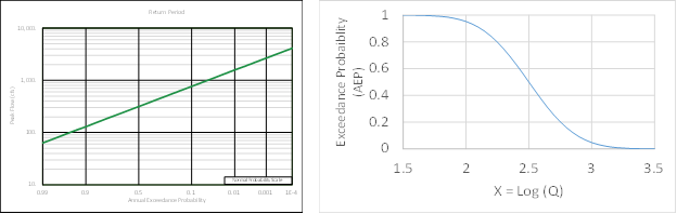
The curve on the left in the figure below shows a typical flow frequency curve plotted using a normal probability scale on the x-axis for AEP and a logarithmic scale on the y-axis for flow. The frequency curve shown on the right is the exact same frequency curve plotted using a linear scale on the y-axis for AEP and a linear scale for Log(Q) on the x-axis.
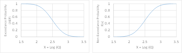
Flow frequency curves are typically plotted as an exceedance curve. Exceedance means the probability that flow is greater than a value. The complement of the flow frequency curve has notation F(x) and is called a non-exceedance curve or a cumulative distribution function which means the probability that flow is less than a value. The two are related by AEP = 1 – F(X). In the figure below, the non-exceedance curve shown on the right is the complement (or mirror image) of the exceedance curve shown on the left. Note that the curve on the right has the classic s-shape of a normal distribution because the logarithm of flow has a normal distribution when the skew is equal to zero.
The probability density function has notation f(x) and can be calculated as the derivative of the non-exceedance curve which means that f(x) = d F(x) / dx. Conversely, the non-exceedance curve can be calculated as the integral of the density function which means that F(x) = ∫ f(x) dx.
The f(x) used in the EMA equations can be derived from the typical flow frequency curve in two steps. First, change the typical frequency (exceedance) curve to a non-exceedance curve by replacing AEP with F(x)=1-AEP. This step is shown in the previous set of Figures that showed AEP and F(x) as a mirror image of each other. Second, take the derivative of the non-exceedance curve to get f(x). A derivative is equivalent to calculating the slope of the non-exceedance curve or the slope of F(x) at every point along the curve. A user defined function is available in the workbooks to calculate f(x).
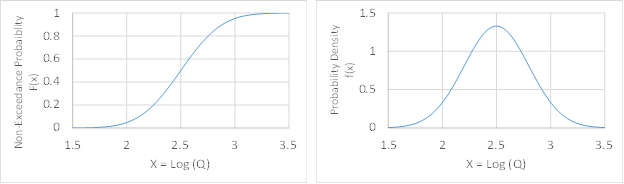
In the figure below, the probability density function shown on the right is the derivative of the non-exceedance curve shown on the left. The curve on the right has the classic bell curve shape of a normal distribution because the logarithm of flow has a normal distribution when skew is equal to zero.
The different types of curves shown in the above examples [ AEP, F(x) and f(x) ] are all the exact same frequency curve plotted in different ways.
For the typical range of skew values encountered in practice, LP3 curves will have a similar shape as the curves in this example because the LP3 is approximately log-normal for nominal skew values on the order of -0.5 to +0.5.
https://en.wikipedia.org/wiki/Cumulative_distribution_function
https://en.wikipedia.org/wiki/Probability_density_function