Download PDF
Download page Task 1: Heterogeneous Sample.
Task 1: Heterogeneous Sample
Start HEC-SSP and open the “extreme_winds” project. You will find the three data sets in the project, shown in the figure below.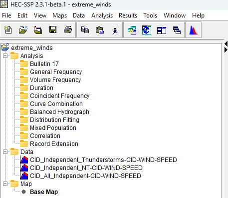
Distribution Fitting Analysis | Partial Duration Series
Create a new Distribution Fitting Analysis (see figure below) and title it “PDS All” (use a description of “partial duration series, all data”) and select the “CID_All_Independent-CID-WIND-SPEED” dataset (see lower figure).


The current dataset contains each independent observation of extreme wind, regardless of meteorological cause, for the period of record. Check to make sure there are no systematic discrepancies in the time-series data by selecting the XY plot type in the lower right corner of the window, as shown below.
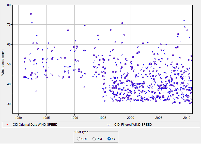
You should see that the minimum recording threshold changed in about 1995. To ensure we are only keeping observations that were measured in the same way for the entire period, use the Filter Data tool, shown below, to drop out observations below 42 mi hr-1 by setting a minimum threshold value.

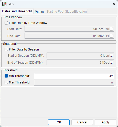
Select OK to apply the minimum threshold. You will notice that the XY plot and the data table now have values in red, which indicate that they were filtered out. Switch to the Analysis tab near the top left of the panel, as shown below. The data in the analysis will be the values that were retained after filtering. You can verify this by selecting the Data Summary Statistics button in the lower left of the panel, which will display various summary statistics for the original and filtered data. Check to see that the minimum value for the “Processed Data” is not below the selected minimum threshold of 42 mi hr-1. Close the Summary Statistics dialog.
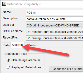

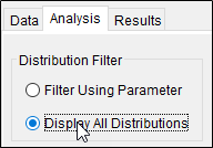
Allow the display of all probability distributions by selecting Display All Distributions under Distribution Filter, as shown below. Normally, this option aids the user by displaying only distributions that are relevant for the kind of data being used (inferred from the DSS information). There are no defaults for wind speed data, so the parameter-based list is a default of commonly used distributions.
Question 1: Based on your knowledge of extreme value theory, which probability distribution would you expect to be a good model for this kind of data (all independent observations of extreme wind speeds)?
Due to the second extreme value theorem, the generalized Pareto distribution should be a good model.
In the Distribution Fitting Methods panel, select the L-Moments (LM) checkbox and uncheck Product Moments (PM).
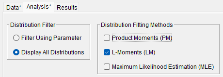
HEC-SSP will immediately compute the estimated probability distribution parameters using the method of L-moments after selecting it. Sort the table by the Kolmogorov-Smirnov (KS) test statistic by clicking on the Kolmogorov-Smirnov (Test Statistic) heading in the table. The best fitting distributions (smallest test statistic) will be at the top of the list. KS is a good default to use and we will keep it.
Question 2: Which probability distribution has the best goodness-of-fit statistic? Is this distribution different from what you were expecting?
The best KS statistic belongs to the generalized Pareto distribution.

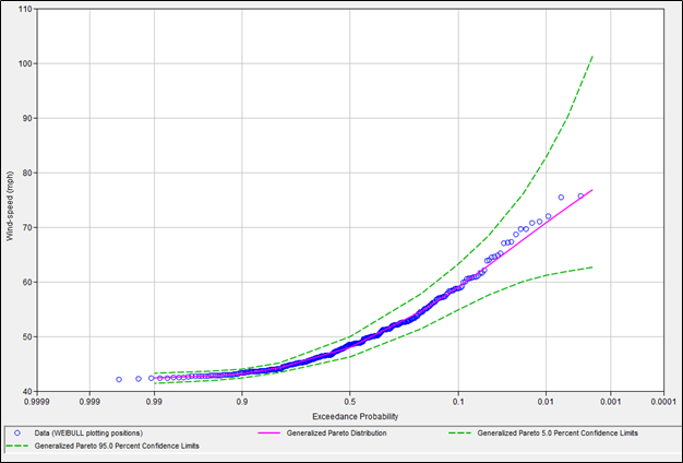
Make sure the plot in the panel uses the CDF-Plotting Position Plot Type (shown below) to show a plot that looks more like a flow-frequency curve.

In the distribution table, select the Generalized Pareto (LM) distribution by selecting the box underneath Median Curve.

Question 3: How do you feel about the goodness of fit based on the “CDF-Plotting Position” plot? Do the data and model show good agreement?
All of the plotted data are well within the confidence limits and are very close to the line representing the estimated model. The Generalized Pareto distribution seems appropriate.
Try some other distributions by turning them on and off in the first column of the distribution table. After looking at the difference between them, return to only having the generalized Pareto distribution selected, and select Accept Selected Distribution on the rightmost column of the Generalized Pareto (LM) distribution in the table.

Select the Results tab.
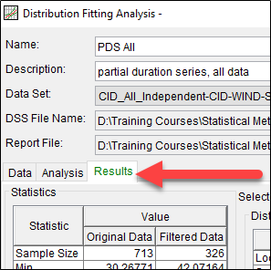
Question 4: Record the location, scale, and shape parameters, as well as the sample size of the filtered data.
All Storm Types – Partial Duration Series Generalized Pareto Distribution (L-moments) | |
Parameter | Value |
Location (ξ) | 42.29455 |
Scale (α) | 8.68748 |
Shape (κ) | 0.15643 |
Sample Size | 326 |
Distribution Fitting Analysis | Annual Maximum Series
Next, we will estimate parameters for the corresponding annual maximum series model. Select OK in the lower right corner of the panel, then save the project.
Create a new Distribution Fitting Analysis and title it “AMS All.” Select the “All Independent” dataset as you did in the first analysis. Instead of filtering out winds below 42 mi hr-1, we will use a filter based on annual maxima. Select the Data Filter tool and on the Peaks tab, select the Filter to Annual Maxima checkbox (shown below). Enter a date of 01Oct (roughly the time of year when storms transition from thunderstorms to mid-latitude cyclones/fronts in this area, and have a slight lull in storm events). Press OK to apply the filter and exit.

Press Apply in the lower right corner and switch to the Analysis tab. Select Display All Distributions under the Distribution Filter. Under Distribution Fitting Methods, select L-Moments (LM) and unselect Product Moments (PM). Sort the resulting distributions by their Kolmogorov-Smirnov (Test Statistic) by clicking on the column header.
Question 5: Based on your knowledge of extreme value theory, which probability distribution would you expect to be a good model for this kind of data (block maxima of wind speeds)?
Due to the first extreme value theorem, the generalized extreme value distribution should be a good model.
Question 6: Which probability distribution has the best goodness-of-fit statistic? Is this distribution different from what you were expecting?
The Gumbel distribution has the lowest KS statistic. The Gumbel distribution is one of the three extreme value distributions so this result is not completely unexpected.

The KS statistic for the top four distributions on the list (Gumbel, generalized logistic, generalized extreme value and log-logistic) are very similar to each other. Compare the difference in behavior of these four distributions by turning their curve display on and comparing their CDF-Plotting Position plots.
Question 7: Which probability ranges of the four models show the most similarity? Where are they the most different?
The four models tend to agree the most within the range of the data (between 0.9 and 0.1 AEP). They diverge the most at the tails.

Question 8: What is special about the relationship between the Gumbel and generalized extreme value distribution? Which would be considered a more “flexible” distribution, and why?
The Gumbel distribution is one of the three cases of extreme value distribution represented by the GEV distribution (GEV becomes Gumbel when the shape parameter is 0). The GEV distribution is more flexible because it has an additional parameter that allows it to take represent three other distributions (the Gumbel, the Fréchet, and the Weibull).
Question 9: Record the location, scale, and shape parameters, as well as the sample size of the filtered data.
All Storm Types – Annual Maximum Series Generalized Extreme Value (L-moments) | |
Parameter | Value |
Location (ξ) | 58.40654 |
Scale (α) | 6.85109 |
Shape (κ) | 0.17483 |
Sample Size | 32 |
Press OK in the lower right to save the analysis. Then, save your project.
Next step: Task 2: Homogeneous Samples