Download PDF
Download page Task 6. Analyze the Flow-Frequency Results.
Task 6. Analyze the Flow-Frequency Results
Statistical analyses can be used to provide estimates of flow (or volume, stage, precipitation, etc.) for extremely rare annual chances of exceedance (ACE), such as 1/10,000. This is common within dam and levee safety studies where a hydrologic hazard curve must be developed that encompasses a wide range of possible hydrologic or hydraulic scenarios. Using the previously created Bulletin 17 and Mixed Population Analyses, you will extrapolate results for very rare ACE and compare the results.
- Open the Mixed_B17C Bulletin 17 analysis.
- Move to the Options tab.
- Within the Output Frequency Ordinates panel, enable the checkbox to Use Values from Table Below.
- Left click, then Right click on the first row and select Insert Row(s)…
- Enter 3 and click OK to insert three additional rows within the frequency ordinates table.
- Enter 0.001, 0.01, and 0.1 within the three new rows. The values within this table must be ascending.
- Click Compute.
- Open the MPA_analytical_curves Mixed Population analysis.
- On the General tab, check the box to Use Values from Table Below within the Output Frequency Ordinates panel.
- Left click, then Right click on the first row and select Insert Rows…
- Enter 3 and click OK to insert three additional rows within the frequency ordinates table.
- Enter 0.001, 0.01, and 0.1 within the three new rows. The values within this table must be ascending.
- Move to the Frequency Curves tab.
- Click the Compute button above the flow-frequency table for both Frequency Curves.
- Click Compute at the bottom of the editor to compute the Mixed Population analysis.
Next, we will visualize the four frequency curves using the spreadsheet provided at the top of this page.
- Open the spreadsheet named "Frequency_Curve_plots.xlsb"
- Click the Curves tab.
- Copy the frequency curve ordinates from the HEC-SSP Mixed_B17C, Summer_Peaks_B17C, Winter_Peaks_B17C, and MPA_Analytical analyses into the appropriate columns.
- Click the Frequency Chart tab to view the curves.
- Use this plot to help answer the next two questions.
Question 3: What are the computed flow rates for the complete range of ACE for both the Mixed_B17C analysis as well as the MPA_analytical_curves analysis? Fill in the following table.
AEP | Flow Rate (cfs) for Analysis: | ||
|---|---|---|---|
Mixed B17C | MPA analytical curves | Difference | |
0.001 | |||
0.01 | |||
0.1 | |||
0.2 | |||
0.5 | |||
1 | |||
2 | |||
5 | |||
10 | |||
20 | |||
50 | |||
80 | |||
90 | |||
95 | |||
99 | |||
AEP | Flow Rate (cfs) for Analysis: | ||
|---|---|---|---|
Mixed B17C | MPA analytical curves | Difference | |
0.001 | 46891 | 70597 | -23706 |
0.01 | 32387.4 | 42062.1 | -9674.7 |
0.1 | 21477.8 | 23965.1 | -2487.3 |
0.2 | 18768.8 | 20073.4 | -1304.6 |
0.5 | 15536.5 | 15857.6 | -321.1 |
1 | 13330.6 | 13274.9 | 55.7 |
2 | 11309.4 | 11108.3 | 201.1 |
5 | 8887.5 | 8713.7 | 173.8 |
10 | 7215 | 7143.4 | 71.6 |
20 | 5644.7 | 5695 | -50.3 |
50 | 3605 | 3790.3 | -185.3 |
80 | 2365.9 | 2579.9 | -214 |
90 | 1918.7 | 2124.3 | -205.6 |
95 | 1622.6 | 1815.1 | -192.5 |
99 | 1200.3 | 1361.1 | -160.8 |
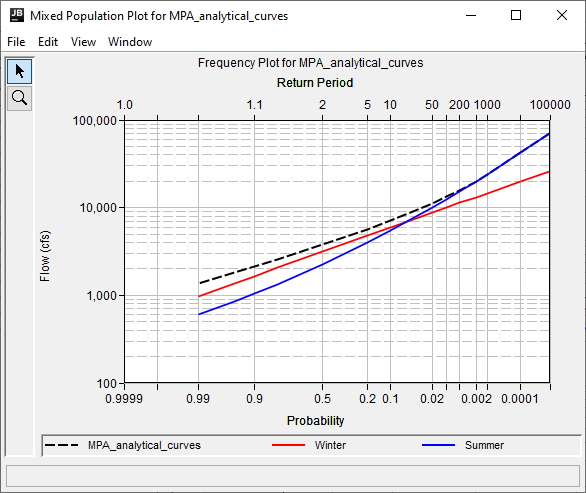
The results of the MPA_analytical_curves analysis is shown in the following figure.

Question 4: What kind of weather/meteorology do you think causes the annual maximum events in each of the seasons? Do you think those types of meteorological events occur every year in this watershed? Do you think they always create the annual maximum discharge for the season? Are the seasonal samples homogeneous?
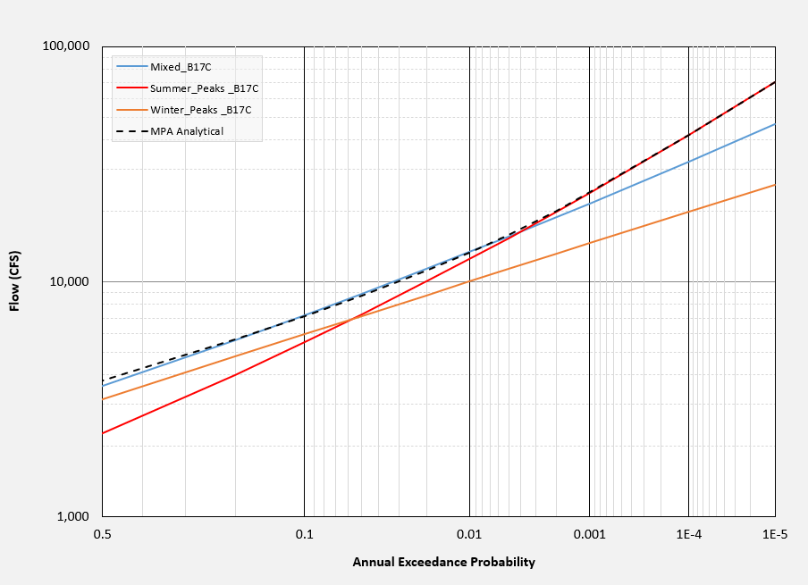
Although the first season is called “winter,” this time period essentially contains the portion of the year that doesn’t fall into the Atlantic hurricane season (typically defined as June 1 – November 30). The precipitation in this season is generally dominated by other large-scale (synoptic) meteorological features (e.g. mid-latitude/extra-tropical cyclones). Generally, many events of this type occur per year. As a result, the probability of receiving a modestly large flood in the wintertime is large. This causes a higher mean and lower variance compared to the “summer” season frequency curve. The summer season generally sees the arrival of tropically-sourced moisture, but as there are few of these events per year anywhere in the Atlantic, there is no guarantee that the largest summer flood in this watershed in each year is tropical in nature. If one of these events does occur in the watershed, however, it is likely to cause extensive flooding (the largest floods in the systematic record at this site were caused by Tropical Storms Agnes [1972] and Ivan [2004]). Smaller summer floods are probably caused by a different mechanism, such as a mesoscale/convective feature, or a tropical event that does not directly fall over the watershed. This is what gives the summer flood frequency curve a higher variance than the winter curve. The seasons are more homogeneous than looking at the annual maximum series naively, but the floods are not all created by the same mechanism. The results from the Summer, Winter, and Mixed_B17C analyses are compared against the results from the MPA_analytical_curves analysis within the following figure.

Question 5. Why did we not use regional skew information in this workshop, particularly in the summer and winter Bulletin 17C analyses?
Regional skew studies are performed using all-season peaks, without consideration of floods of varying causes. Therefore, it is not appropriate to use all-season regional skew information in the summer and winter Bulletin 17C frequency curves. We could have used regional skew information in the mixed Bulletin 17C analysis but we omitted it to produce a uniform comparison between the frequency curves.
Final Project Files

