Download PDF
Download page Task 4. Fit and Compare Multiple Models to the All-Season SWE Time Series.
Task 4. Fit and Compare Multiple Models to the All-Season SWE Time Series
Next, you will fit and evaluate different models to the all-season SWE time series. Again, before fitting any models, use the tools contained within the Distribution Fitting | Data tab to create a representative, independent, and identically distributed sample for this season.
- Create a new Distribution Fitting analysis and name it “LittleMeadows_SWE_AllSeason”.
- Select the Linn-Little Meadows-SWE data set within the Data Set drop down menu.
- On the Data tab, ensure that Other is selected within the Parameter Type drop down and click on the Filter Data button.
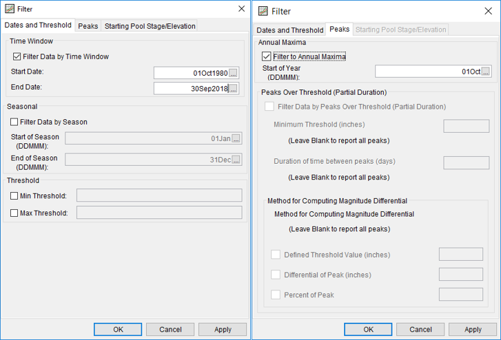
- Within the Filter editor, on the Dates and Threshold tab, click the Filter Data by Time Window box and enter a Start Date and End Date of 01Oct1980 and 30Sep2018, respectively.
- Move to the Peaks tab and click the Filter to Annual Maxima check box. Enter a Start of Year of 01Oct.
- The Dates and Threshold tab and the Peaks tab should appear similar to Figure 1.

- Click OK to apply the filters and close the editor.
Question 12: How many values were contained within the original data set? After applying the filters, how many values remain?
Use the Data Summary Statistics.
Over 15000 values were contained within the original data set. 38 values remain within the filtered/processed data.
Once you are satisfied with the data set, move to the Analysis tab and begin fitting multiple models:
- Click the Apply button in the lower right corner of the Distribution Fitting editor, switch to the Analysis tab, and within the Distribution Filter panel, click the radio button to Display All Distributions.
- Select both Product Moments and Linear Moments (L-Moments) from the Distribution Fitting Methods.
- Try multiple distribution and fitting method choices. Be sure to use the Distribution Fitting analysis’ various plots, tabular data, and tools to visualize each model’s goodness of fit relative to the data. Also, try viewing the PDF, PP Plot, QQ Plot, and CDF-Plotting Position
Question 13: Which distributions provide the best fit to the data? Which fitting method provides the best fit to the data?
Pay close attention to the tail behavior of the models.
There are several models that provide adequate fits to the data including: GLO | Linear Moments, GEV | Linear or Product Moments, Pearson III | Linear or Product Moments, and Gamma | Linear Moments. The differences between these models, when compared to the observed data, are minor. However, not-so-trivial differences can be realized on the tails of each fitted distribution (i.e. when extrapolating beyond the range of the observed annual maximum series). For instance, the Logistic | Product Moments model results in negative SWE values for exceedance probabilities less than approximately 0.95. Similarly, the GLO | Linear Moments model results in negative SWE values for exceedance probabilities greater than approximately 0.99. Also, at first glance, it may appear that the LPIII | Product Moments model provides a reasonable fit to the observed data in addition to extrapolating to more and more likely probabilities. However, when looking at the right tail of the distribution, the model does not fit well and/or predict the exceedance probability of the largest observed SWE accumulation. It is up to the user to explain these issues with estimated values based upon the chosen model.
- Once you have determined an acceptable distribution and fitting method, click the corresponding radio button within the Accept Distribution column. This will compute the confidence limits and expected probability curve (if they weren’t already computed).
- Move to the Results Within this tab, you will find statistics and parameters related to the original data, filtered data, selected distribution and fitting method, selected goodness of fit method, as well as the computed frequency curves.
Question 14: Which model did you choose? What were its parameters? What is the resulting 0.2-, 0.5-, 1-, 2-, and 10-percent chance exceedance SWE for the winter season?
The Gamma | Linear Moments model was chosen for two reasons: 1) it fits the observed data well (made best evident by viewing the model within the PP and QQ plots) and 2) it provides reasonable and defensible extrapolation beyond the range of observed data. However, a case could also be made to choose the GEV | Linear Moments model instead. The shape and scale parameters for this model were 4.330 and 6.929, respectively. The resultant 0.2-, 0.5-, 1-, 2-, and 10-percent chance exceedance all-season SWE magnitudes were 88.3, 79.8, 73.2, 66.4, 57.0, and 49.3 inches, respectively.
- Click the OK button to close the Distribution Fitting analysis editor.
- Click the Save button to save the study.
Continue to Task 5. Compute a Duration Analysis Using the SWE Time Series and Estimate the Required Information.