R is a programming language and environment for statistics and graphics.  The biggest strength of R is its adoption of open-source libraries called packages which make it very easy to add additional functions and features.

R is usually run in an integrated development environment (IDE) such as RStudio.  IDEs simplify many processes for developing code.  RStudio in particular for R gives you tools for managing packages, viewing plots, seeing data and variables that have been defined, executing code, and so on.

There are two typical ways that someone might code in R:

1. At the command line
2. Using scripts

The command line interface (CLI) allows the user to run a line of code at a time and see the result play out.  This can be done with R natively without an IDE, or in the console of an IDE like RStudio.  For simple analyses this can be a very quick way to get a result.  However, for more complicated workflows that will be repeated or reviewed later, the CLI option does not provide an easy way to go back over code that has been run previously.

Scripts are documents that contain a sequence of commands.  The user may choose to run the entire script, in which case each line is fed to the command line and executed until an error occurs or the script completes.  Or, the user may run individual or several lines at a time.  The script is repeatable and reviewable, which makes them useful for studies that will be revisited later.  The script serves as a "receipt" on the analysis, which allows anyone to repeat the analysis and get the same results.

A common method for working in R is to test lines of code at the command line and then add them to the script once their functionality is verified.  This ensures that the programmer knows that a part of the code will work before putting it into their script.

Installation

R and any IDE used to work with it (such as RStudio) need to be installed on your machine in order to work.  This tutorial will show you how to get R and RStudio from the App Portal and ensure it is up and running correctly: Installing and Configuring R and RStudio

Key Concepts

R is a programming language that was designed with statistical analyses in mind.  There are several features fundamental to working with R that might make it different than other programming languages.  Below are several fundamentals to feel comfortable with before beginning your workshops.

Comments

Comments are used to make code more readable. In R, comments start with an octothorpe (#). Text following a # will not be executed.

# This is a comment. Rawr.

Executing Code

There are a number of ways to execute R code:

• Place your cursor anywhere on line of code you want to run and click Ctrl+Enter on your keyboard.
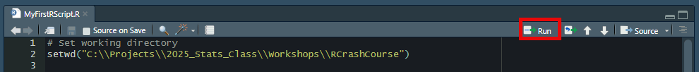
• Click the Run button at the top right of the Script console.
• To execute multiple lines of code at a time, highlight a section of code and use one of the previously described methods.
  

Help

The help function and ? operator can be used to access R documentation pages. 

help(mutate)
?mutate

Variable Assignment

When assigning a value to a variable, R does not use the equals sign (=) (the equals sign is used for something else that we will see later). Instead, R opts for a left-arrow symbol formed by using the less than (<) and minus (-) symbols.  The example below assigns the value 5 to a variable named x.  This code works at the command line or in a script:

x <- 5

Check out this blog if you're interested in learning more about the difference between = and <-.

Persistence of Variables and Default Print Behavior

During a session of R, any variable assignment you make will persist until the session is ended.  This means you can reference variables you created earlier while working.  Any variable assignment adds them to the environment, which is a collection of variables and functions available to the user.  In the Assignment example above, we assigned the value of 5 to the variable x, and if we want to see the value of x later on during our session, we can use the default print behavior to see what we assigned it at any time.

At the command line, entering a variable name triggers its print behavior.  For most types of variable, this means that it will print the value of the variable.  More complex variables may have special display.  For our simple variable x, typing x at the command line and hitting enter will produce the display below.

x
[1] 5

Functions

Functions are fundamental to R.  Functions are repeatable blocks of code that can accept input data to produce an output.  There are many functions available by default with R, but additional functions can be added if they are defined by the user or added via a package.  Functions can be recognized in code by their use of parentheses immediately after a name.  One of the most common and simple functions is the c function (for combine) which takes any number of parameters and returns a collection of the inputs.  The example below shows combining a few numbers into a collection of numbers using the c function, and assigning it to the variable y:

y <- c(3, 5, 7, 9)

The variable y is now a vector containing four values.  Using the default print behavior at the console returns all four values.

y
[1] 3 5 7 9

While R contains many built-in functions, you can create your own functions. An R function is created using the keyword function. A function in R has the following general syntax:

function_name <- function(<arg1>, <arg2>, ...) {
 # Function body
}

 A function is comprised of the following components:

• Function name: The name of the function. The function is stored in R environment as an object with this name.
• Arguments: Arguments are optional placeholders. When a function is called, you pass a value to the argument. 
• Function body: The function body contains statements used to perform a specific task.
• Return value: The return value of a function is the last expression in the function body.

Variables defined within the function body are local variables. These variables exist only within the function. A function can invoke another function.

Variables and Data

The basic data currency for R is the vector.  It is a 1-dimensional array of data where individual values can be accessed by index.  Many functions are vectorized in R, meaning that when you give a vector to a function, it may automatically run that function on each element of the vector and return the result as a new vector the same size as the input.

> y ^ 2
[1] 9 25 49 81
> sqrt(y)
[1] 1.732051 2.236068 2.645751 3.000000

Some functions take multivariate data (such as a vector) and return a single value instead of a vector.

> mean(y)
[1] 6

Some functions take multiple arguments which specify settings or controls.  It is good practice to use the variable names in the function calls, because one or more arguments could be optional and it helps to avoid crossing wires.  This is where the = comes into play.  The function below uses the rnorm function to generate samples from the normal distribution with a specified sample size (n = 50), mean (mean = 100), and standard deviation (sd = 10).  Using the names ensures the right values are provided to the right arguments.

> norm_sample <- rnorm(n = 50, mean = 100, sd = 10)

Accessing Values by Index

One quirk of R that is important to keep in mind is that unlike other programming languages, R counts starting with 1, where most programming languages start at 0.  One positive side effect of this choice is that off-by-one errors are much less common.  One major downside is that people who spend a lot of time in other programming languages will often forget that R counts from 1 instead of 0, and cause themselves an off-by-one error in the other direction.

In a multi-valued data object like variable y in the Functions example above, you can access the individual values using brackets and the number of the item you would like to retrieve.  For example, if you want the third value inside of y, you would type (and R would respond):

y[3]
[1] 7

In other programming languages, entering this would actually give you the fourth value inside of y (because the first value is stored at index 0).

Accessing Values by Name

Some objects store data with names.  Names are another way to access data inside of an object that doesn't require knowing the order of the data.  First, let's create a vector that has three values and store it to a variable called z, and then assign some names.  This process uses the c function to create the initial vector of values.  Then, it uses the "names" function to access the names attribute of z, and assigns a newly-created vector of names to the vector z:

z <- c(2, 4, 6)
names(z) <- c("a", "b", "c")

This turns variable z in to a named vector.  Now, we can access the values by name instead of number as before by using name inside the brackets.  To access the value with name b, we type and R returns:

z["b"]
b 
4 

Certain types of objects can have their named objects accessed a different way, using the dollar sign ($) character.  One example of these objects is the list, which is similar to the vectors created before.  A list's object names can be created in-line when the object is created, shown below.  A list's named objects can be accessed using the dollar sign notation:

w <- list(a=2, b=4, c=6)
w$b
[1] 4

This is useful because some functions return complex objects that have parts that you may want to access.  One example is for linear regression models.  Linear regression returns very complex objects with parts that can be accessed by name, such as the model residuals or fitted values.  This will come in handy later.

Data Frames

Most data are more complex than just a sequence of values.  Often, many observations each with several attributes are collected so that they may be analyzed.  A data frame is an object that holds this type of data.  Observations are stored in rows, and attributes are stored in columns.  Spreadsheet data often look a lot like a data frame.  R contains a small number of demo datasets that are stored as data frames.  One of them is a famous dataset of car data from the 1974 Motor Trend US magazine.  To load this data and print the first five rows of the data frame, use the following:

data(mtcars)
head(mtcars, 5)

The data function tells R to pull up the internal data object called "mtcars" (Motor Trend cars, FYI).  The "head" command tells R to print the first few rows of a data frame. In this case, the second argument specifies the first 5 rows.  You will see a large volume of data printed to the Console, as shown below.

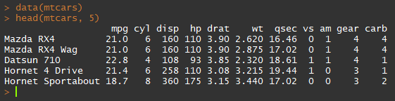
This dataset has 32 rows (observations) and 11 columns (variables).  The first column that has been printed is the row name (this data frame uses the name of the car as the row name).  The data inside this data frame can be accessed in a number of ways.  One of the most common ways is to access a single column, either by number or name.  The following two commands do the same thing, accessing the first column which is called mpg:

mtcars$mpg
mtcars[,1]

The notation of the second command in the Data Frames 2 example shows how data with more than one dimension can be accessed by index.  R uses row/column notation.  If you wanted the first row, you would enter:

mtcars[1,]

If you wanted the value at the sixth row and fifth column, you would enter:

mtcars[6,5]

Data frames also work with access by name.  If you wanted the value of the mpg variable for the row named Datsun 710, you could enter:

mtcars["Datsun 710","mpg"]

Note

Not every data frame uses row names.  This is an optional feature that is used based on preference.  Often, the only way to access a row is by number.

Code Style and Formatting

It's good practice to keep lines of code under 80 characters wide when possible, but sometimes when stringing together complicated workflows it's easy for lines to be hundreds of characters long.  R can break up complicated lines and interpret them as single functions even if they spill over.  It is good practice to break after simple operators like + or *, at commas, after the assignment character <-, after pipes %>%, etc. when it is necessary to do so due to line length.  This can also make code more readable, for example when filling a vector with data:

fruit <- c("banana",
           "watermelon",
           "apple",
           "orange",
           "grape",
           "mango",
           "plantain",
           "tangerine")

Code Organization

R Coding Practices: Organization

In general it is good practice to organize your script so that others can easily follow and read it.

Using white space to break up groups of related commands makes the code easier to read.  I tend to place extra blank lines between groupings like library calls, setting the working directory, loading data, etc.

You can insert a coding section using Ctrl+Shift+R to keep scripts organized.

Placing library calls at the beginning of the script ensures that when it is run, all of the commands have the necessary functions loaded.  It also instructs someone that they might have to install packages if they don't have them already.

Placing the setwd directory at the beginning of the script lets someone else running the script know that they will need to change that directory to make it run on their machine.

Loading all of the necessary data near the beginning of the script ensures it is always available and ready to go after that.

Lines of R code can be broken up so that they don't get so long that they can't be read.  Some functions take a large number of parameters so it can make a function call easier to read to break up the parameters after commas.

Functions are typically defined at the beginning of a file since they must be defined before they can be called. An argument is a value provided to a function to obtain a result.