Download PDF
Download page Phase 3: Model Construction Using R.
Phase 3: Model Construction Using R
In this phase, construct your three (or fewer) predictor model with the appropriate transformations in place for the predictors and/or the response variable. During this phase, you will need to return to the parameter selection process and choose different parameters to make improvements to your model.
To fit a model, you will use the lm() function. This function requires two parts: the data it's using and a formula that describes the model structure. Since we are using pipes, we will specify our data using the dot (.) notation just like in the example below. The formula for typical multiple linear regression is structured with a squiggle (~) between the response variable and the predictors, and a plus (+) sign is used to join the predictors together:
lm Example
lm(data = ., <response> ~ <predictor_1> + <predictor_2> + ...)You will want to store the results of your model fit in a variable so that you can use the summary() function to see the model summary table. The example code below shows how to combine data transformation using mutate(), filter data using select(), fit a model using lm(), and get the model summary. Note that this code will not run because it has placeholders for your transformations, variables, and model formula. The summary() function produces the standard regression output table, including things like the values of the coefficients, the predictor p-values, the model's adjusted R2, and so on.
Model construction
model_1 <-
  fitting_data %>%
  mutate(<YOUR TRANSFORMATIONS HERE>) %>%
  select(<YOUR LIST OF VARIABLES HERE>) %>%
  lm(data = ., <YOUR MODEL FORMULA HERE>)
summary(model_1)After fitting the model, you should evaluate the quality of the fit. A few typical summary statistics that help identify whether or not the model has any power:
- Adjusted-R2: this statistic describes the percent of the variance in the response variable explained by the predictors, adjusting for the model complexity. Each additional parameter reduces adjusted-R2, so adding the variable must be “worth it” by overcoming its penalty. This value is shown in the bottom right of the model summary, in the second-to-last line. With the available data in this data set and use of transformations, you should be able to achieve an adjusted-R2 of at least 0.5.
- P-value for the F statistic: this measures whether or not the proposed model is significantly different than an intercept-only model (smaller p-values are better). If your F statistic p-value is not less than 0.05, it is very unlikely any of your predictors will be significant. Check this value in the last line of the model summary, at the very end of the report.
- If your model F statistic is significant but none of the predictors are, this can be an indication that your predictors are highly correlated with each other. This violates the assumption that they are independent. We will see another tool for checking this assumption in Phase 4.
- Predictor p-value: this measures whether or not the coefficient of your regression is significantly different from zero. The “magic” level is usually p < 0.05; however, many useful models can be constructed with larger p-values, especially if they are still close to 0.05. A p-value greater than 0.1 is starting to get very large. This value can be found in the last column of the Coefficients table in the model summary report. Do not worry about the p-value of the regression constant (a.k.a. the intercept term). The interpretation of the model constant can be difficult, especially in models with extensive transformation. Models with standardized variables should have an intercept at zero.
In a dataset with a limited number of predictors (7 isn't too unwieldy) you can fit a "kitchen sink" model as an initial method for screening your predictor variables. To do this, set up a model that predicts t with a combination of all seven parameters. If any transformations are important for the predictor or response, use that instead of the original predictor/response value. This will give you an idea of where the upper bound on a model R2 could be for these data. You already know that a lot of these predictors are highly correlated with each other and this model will not pass our assumption checks, so we will need to dial back what is included in the final model. However, you may see that some parameters have more power of prediction than others when combined with all the others and may help you focus on a smaller number of predictors at first. The summary below is for a kitchen sink model with no transformations. You can try variations that include transformations (at least one produces an even higher adjusted-R2) but don't spend too much time on this step. Included is a summary of predictor variance inflation factors, a metric we will use in Phase 4 to explore multicollinearity.
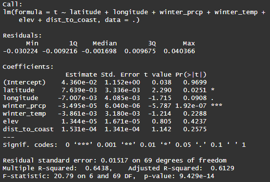
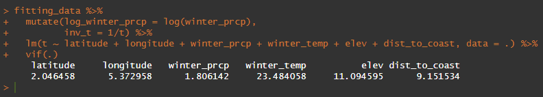
As we will see in Phase 4, the VIF values for these predictors are quite high, with the exception of winter_prcp. It is also the predictor with the smallest p-value in the kitchen sink model. It's probably important.
Record some of your model fits below in Table 1 (use more space if you need to record more model fits). Record the model adjusted-R2, the F-statistic p-value, the transform for the response variable if you used one, the predictor variable and transform for each predictor (up to 3), and the p-value for each. Once you have a model with an adjusted-R2 of at least 0.5, then start checking model assumptions for each of your fits as you seek to improve the model. Save your top regression model results as you will be using this information in the Phase 4. Note: this is not a rule for every model. Some data might achieve an adj-R2 of 0.5 very easily, and some data may never. For this set of data, it is a good place to start checking your model fits.
Table 1. Multiple linear regression models.
Model | Adjusted-R2 | F | Response | Predictor 1 | p-val | Predictor 2 | p-val | Predictor 3 | p-val |
1 | |||||||||
2 | |||||||||
3 | |||||||||
4 | |||||||||
5 | |||||||||
6 | |||||||||
7 | |||||||||
8 | |||||||||
9 | |||||||||
10 |
Go to the Next Step: Phase 4: Checking Assumptions Using R