Multicollinearity and residual normality tests for the three models are shown in Table 1.

Table 1.  Checking results for regression models.

The VIFs for model #1 are elevated but not worryingly high (the maximum is well below 2.5).  The VIFs are nearly 1 for the other models after dropping latitude as a predictor (1 is the minimum value possible for VIF.)

Shapiro-Wilk tests on all three models’ residuals fail to reject the null hypothesis of normality.

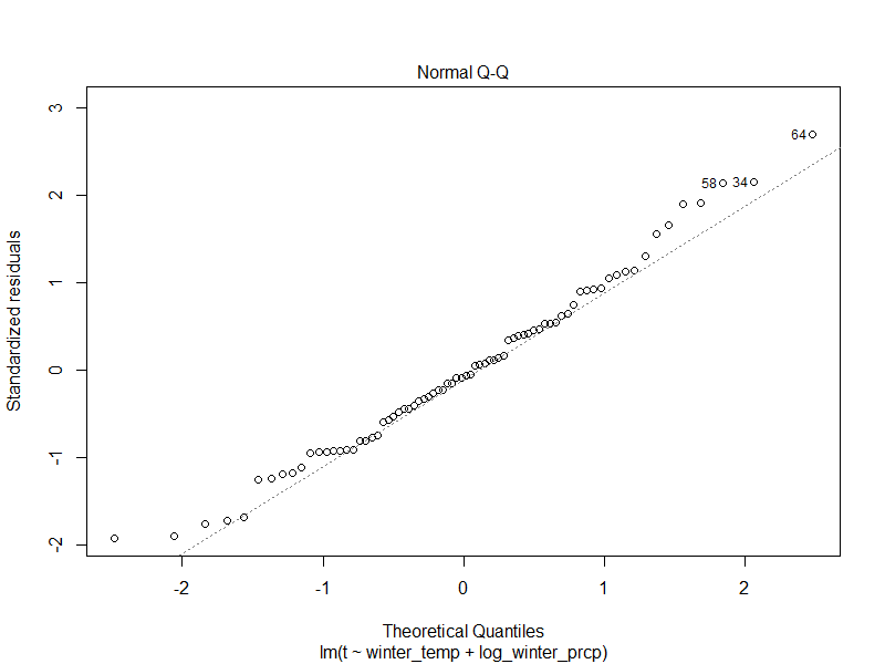
The Q-Q normal plot for model #1 is shown Figure 1 below.  It shows reasonable normality with a slightly concerning curl upwards both tails.  The Shapiro-Wilk test fails to reject the hypothesis of normality so this is not as concerning.

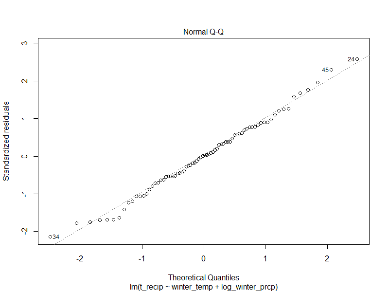
Figure 2 shows the normal Q-Q plot for model #2, which agrees well in the middle of the distribution with some overprediction in the tails.  However, the Shapiro-Wilk suggests this behavior is ok.

The residual normal Q-Q plot in Figure 3 is for model #3.  This shows excellent behavior in terms of normality of the residuals.

Final Model

Model #2 was selected as the “final” one, although other useable models using these data are likely to exist.  Model #2 was selected over model #1 because the latitude predictor was not significant (and #1 had higher even if not remarkable VIFs) even though its adjusted-R² was higher.  The latitude predictor is in a grey area where it contains information about t but the evidence is not strong enough to suggest it is meaningful.  In a real study, it would be worthwhile to try to find more data, perhaps the physical phenomenon that latitude is trying to explain.  Model #3 had better properties for its residuals but a worse adjusted-R² than model #2. However, since the Shapiro-Wilk test failed to reject the normality hypothesis for model #2, the loss in adjusted-R² wasn’t worth the additional improvement to the residuals.

Question 3: How well does the model perform out of sample?  Is this performance better or worse than you expected?  Which observations are predicted well?  Which are predicted poorly?

Using the model above (note that your model and therefore answer may be different) there are 5 observations (out of 28) that fall outside the 95% prediction interval (open the validation_data_with_model_2.pi data frame).  This means that the model prediction interval set to 95% only covers about 82% of the validation dataset, which is less than expected.  The 5 sites with the highest predicted error don't seem to have any characteristics measured by the other data that make them stand out (e.g. the site consistently at high elevation).  Using the model above, and plotting the prediction error at the validation sites against other variables shows weak linear relation with a couple variables, winter temperature and distance to the coastline (which themselves are highly correlated with each other).  The model performance on the validation sites can be measured using RMSE (root mean square error) which is computed by taking the average of the square of the errors, then taking the square root.  The model above has an RMSE of about 0.0245 on the validation set, which we can use as a baseline for comparing other model structures.  

Question 4 (time permitting): Is there a predictor variable that if added to the original model, would improve the prediction of those sites in the validation set that were predicted poorly?

First by transforming the winter temperature by squaring it, the adjusted-R² in the fit increases an unremarkable amount (up to 0.6309) but the prediction interval coverage is unchanged, and the validation RMSE decreases an unremarkable amount.  Trying to add the distance to coastline variable runs into some issues.  First, the predictor is not significant in the initial model fit, and it decreases the adjusted-R².  When checking for multicollinearity, the VIFs for the model blow up - winter_temp and dist_to_coast are highly collinear (VIF > 4.3).  We could have anticipated this in looking at the scatterplots before.  Forging ahead with this model, we find that we still have not improved the prediction interval coverage on the validation dataset, although the validation RMSE does decrease, albeit a tiny amount.  Checking the performance of model #1 above, which includes the latitude term, does not improve the PI coverage, and only very slightly reduces the validation RMSE.  It is unfortunate that we are unlikely to be able to improve this model's performance on the validation dataset.