Download PDF
Download page Analyzing Probability Distributions.
Analyzing Probability Distributions
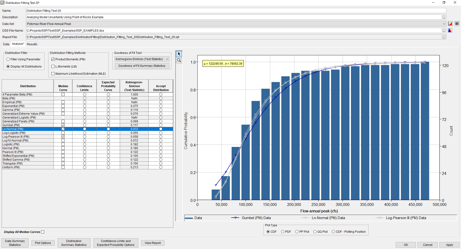
Once the data set has been analyzed and accepted, the user can begin to analyze multiple probability distributions and fitting methods within the Analysis tab. As shown in Figure 1, the Analysis tab contains settings, information, and options related to the available frequency distributions and fitting methods that will be used to generate the results. These settings include:
- Distribution Filter
- Distribution Fitting Methods
- Goodness of Fit Test
- Distribution | Fitting Method Table
- Data Summary Statistics
- Distribution Summary Statistics
- Confidence Limits and Expected Probability Options
- Plots
Distribution Filter
This option allows the user to change the listing of distributions that will be available within the Distribution | Fitting Method Table. When the Filter Using Parameter option is selected, only those distributions commonly associated with the chosen Parameter Type on the Data tab will be available. When the Display All Distributions option is selected, as shown in Figure 2, all currently available probability distributions will be shown.

Distribution Fitting Method
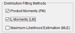
Three distribution fitting method choices are available for use: Product Moments (PM), L-Moments (LM), and Maximum Likelihood Estimation (MLE). Multiple distribution fitting methods can be selected at the same time, as shown in Figure 3.
Goodness of Fit Test
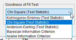
Five goodness of fit tests are available for use: Kolmogorov-Smirnov, (Pearson's) Chi-Square, Anderson-Darling, Bayesian Information Criterion, and Akaike Information Criterion. A goodness of fit test can be selected from the drop down menu, as shown in Figure 4. The goodness of fit tests will present results in terms of a test statistic. It is up to the user to interpret these results for their specific application.
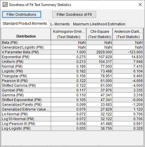
Goodness of Fit Summary Statistics
The Goodness of Fit Summary Statistics button, which is available as a button under the Goodness of Fit Test section, can be used to summarize the goodness of fit test statistics for all of the distribution | fitting method combinations (Figure 5). Tabs for Standard Product Moments, L-Moments, and Maximum Likelihood Estimation are included. The Filter Distributions button allows the user to include or remove distributions from the results. The Filter Goodness of Fit button allows the user to include or remove goodness of fit tests from the results. The Goodness of Fit Summary Statistics window is shown in Figure 6. The contents of the table can be sorted in ascending or descending order using the computed goodness of fit test statistic by selecting the corresponding column header.

Distribution | Fitting Method Table
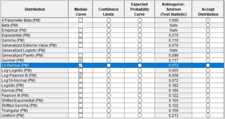
The Distribution | Fitting Method table contains a list of the available distributions, options to display and/or compute various curves, options to change the fitting method, and goodness of fit test statistics for each distribution | fitting method, as shown in Figure 7. The contents of the table can be sorted in ascending or descending order using the computed goodness of fit test statistic by selecting the Test Statistic column header. Not all distribution | fitting method combinations will converge to and result in real-space parameter estimations when subjected to different data sets. Distribution | fitting method combinations that do not converge will be greyed out and not available for selection. The user can also interact with the available distribution | fitting method combinations in several ways:
- Display Median Curve
- Display Confidence Limits
- Display Expected Probability
- Goodness of Fit Test Statistic
- Accept Distribution
Median Curves
The Median Curves option, which is available as a checkbox within the left-most column header, can be used to display and/or remove the median curves for each distribution that is currently shown in the Distribution | Fitting Method table within the currently selected plot type. Alternatively, the Display All Median Curves option, which is available as a checkbox in the lower left of the Analysis tab, can be used to display and/or remove median curves for all distributions that are currently shown in the Distribution | Fitting Method table within the currently selected plot type.
Display Confidence Limits
The Display Confidence Limits option can be used to display and/or remove the confidence limits for the selected row / distribution within the currently selected plot type. Options controlling the confidence limit computations and results are contained within the Confidence Limits and Expected Probability Options menu.
Confidence limits cannot be plotted within the PDF, PP, and/or QQ plot. In addition, only one set of confidence limits can be displayed at a time. When this button is pressed, if the confidence limits for the selected distribution | fitting method have not been computed, they will be computed prior to display. If the confidence limits for the selected distribution | fitting method have previously been computed, they will be displayed without being recomputed. In addition, if the parametric bootstrap computations that estimate the confidence limits fail to converge using the specified convergence criteria, an error message will be shown stating, "Compute failed to converge." If this error message is encountered, please check the specified convergence criteria. However, the Results tab will still be populated with the available information.
Display Expected Probability
The Display Expected Probability option can be used to display and/or remove the expected probability (mean) curve for the selected row / distribution within the currently selected plot type. Options controlling the expected probability computations and results are contained within the Confidence Limits and Expected Probability Options menu.
Expected probability curves cannot be plotted within the PDF, PP, and/or QQ plot. In addition, only one expected probability curve can be displayed at a time. When this button is pressed, if the expected probability curve for the selected distribution | fitting method has not been computed, it will be computed prior to display. If the expected probability curve for the selected distribution | fitting method has previously been computed, it will be displayed without being recomputed. In addition, if the parametric bootstrap computations that estimate the expected probability curve fail to converge using the specified convergence criteria, an error message will be shown stating, "Compute failed to converge." If this error message is encountered, please check the specified convergence criteria. However, the Results tab will still be populated with the available information.
Goodness of Fit Test Statistic
The Test Statistic column shows the computed test statistic for the selected goodness of fit test. The contents of the table can be sorted in ascending or descending order using the computed goodness of fit test statistic by selecting the Test Statistic column header.
Accept Distribution
This Accept Distribution radio buton allows the user to accept the currently selected distribution and populate the Results tab with relevant output.
When a distribution has been accepted, the selected distribution | fitting method combination row will be highlighted in green, as shown in Figure 8.
When this button is pressed, the confidence limits and/or expected probability curve for the selected distribution | fitting method will be computed (if they have not been computed already). If the confidence limits and/or expected probability curve for the selected distribution | fitting method have previously been computed, they will be displayed without being recomputed. In addition, if the parametric bootstrap computations that estimate the confidence limits and expected probability curve fail to converge using the specified convergence criteria, an error message will be shown stating, "Compute failed to converge." If this error message is encountered, please check the specified convergence criteria. However, the Results tab will still be populated with the available information.
Data Summary Statistics
The Data Summary Statistics button is located in the lower left-hand corner of the Analysis tab. The button will launch a window that contains summary statistics for both the original data and processed data.
Distribution Summary Statistics
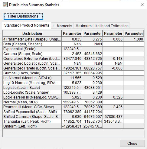
The Distribution Summary Statistics button is located on the bottom of the Analysis tab. The button will launch a window that contains the distribution parameters for each distribution | fitting method combination. Tabs for Standard Product Moments, L-Moments, and Maximum Likelihood Estimation are included, as shown in Figure 9. The displayed distributions can be filtered by selecting the Filter Distributions button.
Confidence Limits and Expected Probability Options
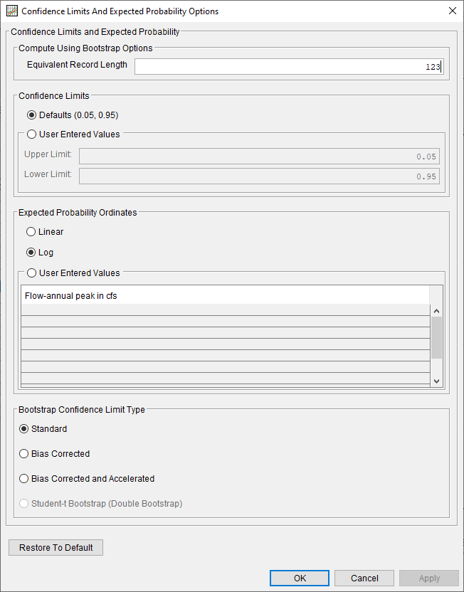
Clicking the Confidence Limits and Expected Probability Options button will launch an editor that contains several options pertinent to the parametric bootstrap routine used to estimate confidence limits and expected probability curves for each distribution | fitting method combination. Three bootstrap confidence limit (and expected probability) computation types are available for use: Standard, Bias Corrected, and Bias Corrected and Accelerated. The Standard method (also known and the Percentile Bootstrap method) computes confidence limits and an expected probability curve using the following algorithm (Efron, 1982):
- Using the initially fitted model produced by the chosen fitting method | distribution, extract a sample of size equal to the Equivalent Record Length.
- Using the same fitting method, fit the same distribution to the sample to produce a new fitted model.
- Randomly sample a single value from the new fitted model.
- Save values corresponding to flow/stage/etc at each of the Output Frequency Ordinates specified within the Plot Options window.
- Repeat 10000 times.
- Sort the values and build a representative histogram to store the values.
- This histogram can be defined using linear, log, or user defined values.
- By default, linear values will be used.
Confidence limits and expected probability curves produced using the Standard method are considered 1st order accurate. The Bias Corrected method uses a bias-correction factor to correct for bias in the skewness of the estimates obtained through the Standard method (Efron and Tibshirani, 1993). The Bias Corrected and Accelerated bootstrapping method improves upon the Bias Corrected method by introducing an acceleration constant that uses jackknife sampling, or sampling without replacement, to estimate parameters. Confidence limits and expected probability curves produced using either the Bias Corrected or Bias Corrected and Accelerated methods are considered 2nd order accurate (McCullough and Vinod, 1998). The Confidence Limits and Expected Probability Options window is shown in Figure 10.
Plots
Plot settings can be modified by clicking the Plot Options button, located on the bottom of the Analysis tab. The following plot options are available: Output Labeling, Plotting Position, Output Frequency Ordinates, and Advanced Histogram Options. The Advanced Histogram Options only affect the PDF plot. The Plot Options window is shown in Figure 11.
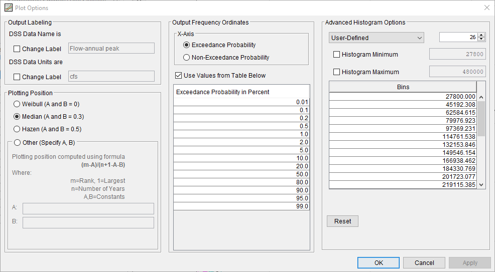
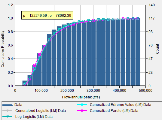
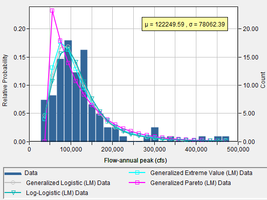
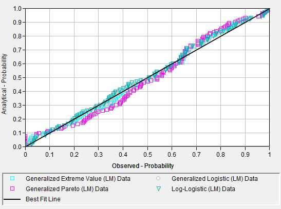
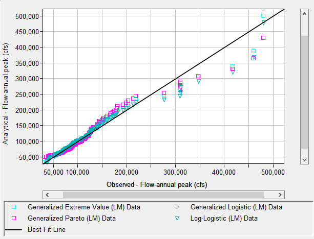
Five different plot types are available for use within the Analysis tab: CDF, PDF, PP, QQ, and CDF-Plotting Position. The CDF plot displays the cumulative histogram of the data in addition to the median, confidence limits, and/or expected probability curves of the distribution(s), as selected and/or computed by the user. The PDF plot displays the histogram of the data in addition to the median curve(s) of the distribution(s), as selected by the user. Within both the CDF and PDF plots, a legend will display the sample mean (μ) and standard deviation (σ) of the processed data. If the user wishes to modify the number or size of the bins used within the either the CDF or PDF plots, the changes should be made on the Data tab. This will ensure that the analytical distributions shown within either plot are the most up to date. The PP plot displays the empirical probability of the data (using the chosen plotting position formula) against the inferred (analytical) probability derived from the distribution | fitting method combination. The QQ plot displays the data against the inferred (analytical) values derived from the distribution | fitting method combination. Both the PP and QQ plots contain a 1:1 line and utilize linear x- and y-axes. Finally, the CDF-Plotting Position plot displays the empirical probability of the data (using the chosen plotting position formula) in addition to the median curve, confidence limits, and/or expected probability curves, as selected and/or computed by the user. This plot utilizes a normal probability x-axis. Examples of all five plot types are shown in Figure 12, Figure 13, Figure 14, Figure 15, and Figure 16.
