Download PDF
Download page Duration Analysis General Settings and Options.
Duration Analysis General Settings and Options
Once the analysis name and data set are selected, the user can begin defining the analysis. Contained on the Duration Analysis editor are four tabs. The tabs are labeled General, Options, Results, and Manual Entry. This section of the manual explains the use of the General and Options tabs.
General
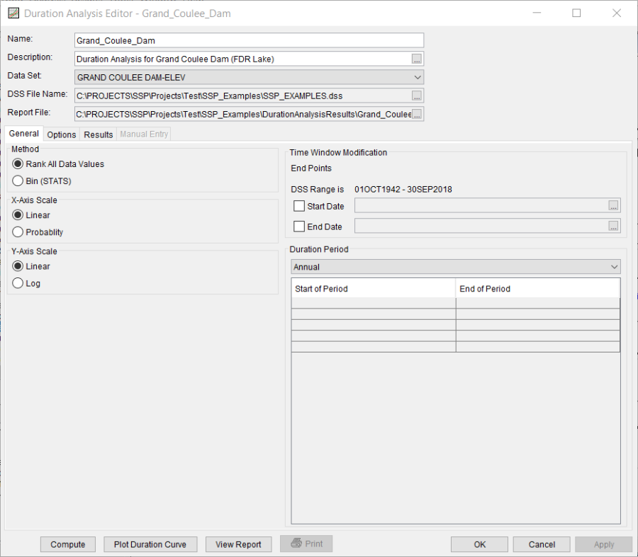
The first tab contains general settings for performing the duration analysis (Figure 1). These settings include:
- Method
- X-Axis Scale
- Y-Axis Scale
- Time Window Modification
- Duration Period
Method
This option allows the user to choose the Rank All Data Values or Bin (STATS) method for computing the duration analysis as shown in Figure 2; the rank all data values method is the preferred choice. This method computes the duration curve by sorting the data from largest to smallest, ranking the values from 1 to n, and using the generalized plotting position formula. The Bin method uses a similar procedure as in the STATS program for computing the duration curve (U.S. Army Corps of Engineers, 1996). The data is grouped into bins (classes) and the duration curve is computed using the number of data in each bin.

X-Axis Scale
This option allows the user to choose the scale of the x-axis. The options are Linear and Probability, as shown on Figure 3. This option will affect the x-axis scale in the duration curve plot and how the "interpolated" frequency curve is computed. The program will use a probability scale when interpolating the final duration curve to the user specified exceedance ordinates.

Y-Axis Scale
This option allows the user to choose the scale of the y-axis. The options are Linear and Log, as shown on Figure 4. This option will affect the y-axis scale in the duration curve plot, how the program computes evenly spaced bins when the Bin (Stats) method is selected, and how the "interpolated" frequency curve is computed. One option for computing bins is to let the program define the bins at evenly spaced intervals between the minimum and maximum values from the selected data set. When Log is set as the y-axis scale, the program will convert the minimum and maximum values to log space before computing the evenly spaced bin limits. Also, the program will use log scale when interpolating the final duration curve to the user specified exceedance ordinates.

Time Window Modification
This option allows the user to narrow the time window used for the analysis (Figure 5). The default is to use all of the data contained in the selected data set. The user can enter either a start date for the analysis, and end date, or both a start and end date. If a start and/or end date are used, they must be dates that are encompassed within the data stored in the selected data set. The date range for the selected data set is shown in the editor just above the Start Date field.

Duration Period
This option allows the user to compute multiple duration curves for different time windows within the year, as shown in Figure 6. If Annual is selected, then the program uses all the data when computing the duration curve. If Quarterly is selected, then the program separates the data into quarters and computes a separate duration curve for each quarter. For example, a duration curve for the 1st quarter includes all data measured from Jan 1 – March 31. The program will compute a separate duration curve for each month of the year when the Monthly option is selected. The User-Defined option lets the user define one or multiple periods within the year. Then the program will perform the duration analysis using data only measured during the user-defined period(s).

Options
In addition to the general settings, there are also several options available to the user for modifying the computations of the duration curve. These options include:
- Output Labeling
- Plotting Position Formula
- Interpolated Curve
- Output Frequency Ordinates
- Bin Limits
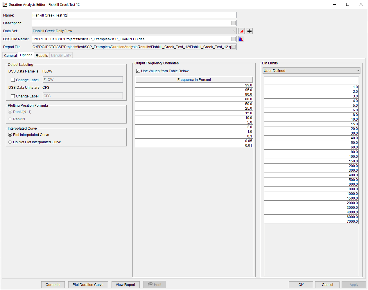
When the Options tab is selected, the Duration Analysis editor will appear as shown in Figure 7.
Output Labeling
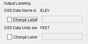
This option (Figure 8) allows the user to change the default labels for data contained in the output tables and plots. The user can change both the name of the data as well as the units of the data. The output labeling does not result in the conversion of data from one unit system to another; it only affects what is displayed on table headings and the y-axis of the results plot.
Plotting Position Formula
This option allows the user to choose how the duration curve is computed, as shown in Figure 9 (this option is not available when the Bin method is selected).

When Rank/(N+1) is selected the program will compute the duration curve by sorting the data from largest to smallest, ranking the values from 1 to n, and using the generalized plotting position formula and Weibull criteria:
P=100 * \frac{m}{(n+1)}
where: m= rank of values with the largest equal to 1.
n= number of values in the data set.
When Rank/N is selected the program will compute the duration curve using:
P=100 * \frac{m}{n}
where: m= rank of values with the largest equal to 1.
n= number of values in the data set.
Interpolated Curve
This option allows the user to plot or not plot an interpolated curve, as shown in Figure 10.

Output Frequency Ordinates
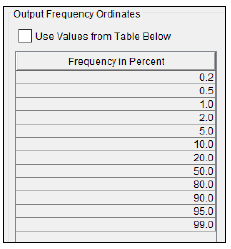
This option allows the user to change or add to the frequency ordinates for which the resulting frequency curve and confidence limits are computed. The default values listed in percent chance exceedance are 0.2, 0.5, 1, 2, 5, 10, 20, 50, 80, 90, 95, and 99, as shown in Figure 11. Check the box next to Use Values from Table below to change or add additional values. Once this box is checked, the user can add/remove rows and edit the frequency values. To add or remove a row from the table, select the row(s), place the mouse over the highlighted row(s) and click the right mouse button. The shortcut menu contains options to Insert Row(s), Append a Row, and Delete Row(s). The program will use the default values, even if they are not contained in the table, when the Use Values from Table below option is not checked. Finally, all values in the table must be between 0 and 100. Note that these values have no impact on the computed frequency curve, but rather only the values of the curve that are reported.
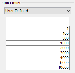
Bin Limits
The Bin Limits panel is only active when the Bin (STATS) method is selected on the General tab. This option helps the user to define the limits, the minimum and maximum values, for each bin. There are two options; Evenly Spaced and User-Defined. When Evenly Spaced is selected the user must also enter the number of bins. The Extract Bin Limits button will automatically populate the bin limits table by first extracting the minimum and maximum values from the data set and then linearly interpolating evenly spaced bin limits. If Log is selected as the Y-axis scale on the General tab, then the program converts the minimum and maximum values to log space before computing the evenly spaced bin limits. The User-Defined option, shown in Figure 12, lets the user manually enter the bin limits. The user must ensure the minimum and maximum values from the data set are contained in the bin limits table. For example, if the minimum flow from the data set is 100.0 then the first row in the table must be less than or equal to 100.0. Additional rows can be added to the table. Place the mouse pointer on top of the table and click the right mouse button. Then select the Insert Row(s)… menu option to open an editor for specifying the number of rows to insert into the table.
