Download PDF
Download page General Settings for Mixed Population Analysis.
General Settings for Mixed Population Analysis
Once the analysis name has been entered, the user can begin defining the analysis. Contained on the Mixed Population Analysis editor are three tabs. The tabs are labeled General, Frequency Curves, and Results. The first tab contains general settings for performing the Mixed Population Analysis. These settings include:
- Number of Curves
- Extrapolate Input Data
- Output Labeling
- Log Transform
- Data Type
- Confidence Limits
- Output Frequency Ordinates
Number of Curves
This option lets the user choose the number of input frequency curves that will be used to compute a mixed population frequency curve as shown in Figure 1. The Frequency Curves tab will update based on the number of curves specified in this panel.

Extrapolate Input Data
This option allows the user to choose whether the imported data may be extrapolated during the mixed population computations as shown in Figure 2. When using either imported results from an Existing Analysis or Manual Entry, the computations will not extrapolate input data, by default. If one or more input frequency curves do not contain enough information to compute a mixed population curve for the specific output frequency ordinates, the results will be left blank. When this extrapolation of the input data is allowed (and imported results from an Existing Analysis and/or Manual Entry are being used), a probability of 1.0 will be assumed for all values that are less than the smallest entered value. Conversely, a probability of 0 will be assumed for all values that are greater than the largest entered value. When using analytical distributions, extrapolation can be performed automatically.

Output Labeling
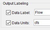
This option, shown in Figure 3, allows the user to enter labels for data contained in the output tables and plots. The user can enter the name of the data as well as the data units. The output labeling does not result in the conversion of data from one unit system to another; it only affects what is displayed on table headings and the y-axis of the results plot.

Log Transform
There are two options contained within the Log Transform setting as shown in Figure 4: Use Log Transform and Do not use Log Transform. This setting only affects the y-axis of subsequent plots. If the user selects Use Log Transform, the y-axis of all plots will use a logarithmic scale (base 10). If the user selects Do Not Use Log Transform, the y-axis of all plots will use a linear scale. This option does not affect any of the computations. The default setting is Do Not Use Log Transform.

Data Type
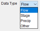
The Data Type selection is used, in conjunction with the settings on the Tools | Options | Results tab, to define the precision of tabular data on both the Frequency Curves and Results tabs. In addition, the Data Type is used (in conjunction with the Equivalent Years of Record option) to compute confidence limits (when requested by the user) using the order statistics method that is discussed in ETL 1110-2-537. The default Data Type is Flow. To select a different data type, click the drop down menu and select either Stage, Precip (Precipitation), or Other (Figure 5).

Confidence Limits
The computed mixed population curve is only an estimate of the probability distribution of the larger parent population. Confidence limits can be used to provide a measure of the uncertainty of the estimated exceedance probability of a selected discharge, stage, precipitation depth, etc. or a measure of the uncertainty of the discharge, stage, precipitation depth, etc. at a selected exceedance probability.
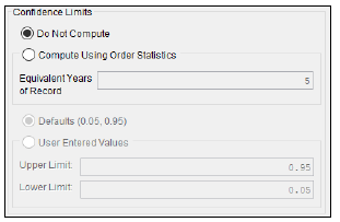
By default, confidence limits will not be computed within a Mixed Population Analysis. However, the user has the option to compute confidence limits using the order statistics method, which is discussed in ETL 1110-2-537. The Equivalent Years of Record must be defined when using this method. (See Figure 6.)
When computing confidence limits, the default interval will be 90 percent confidence (i.e. the 5% and 95% confidence limits). The confidence limits must be entered in decimal form (i.e. 95% = 0.95, and 5% = 0.05). The user has the option to override the default values and enter whatever values they would like for the confidence limits.

Output Frequency Ordinates
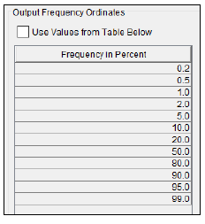
This option allows the user to change or add to the frequency ordinates for which the resulting frequency curve and confidence limits are computed, as shown in Figure 7. The default values listed in percent chance exceedance are 0.2, 0.5, 1, 2, 5, 10, 20, 50, 80, 90, 95, and 99. Check the box next to Use Values from Table below to change or add additional values. Once this box is checked, the user can add/remove rows and edit the frequency values. To add or remove a row from the table, select the row(s), place the mouse over the highlighted row(s) and click the right mouse button. The shortcut menu contains options to Insert Row(s), Append a Row, and Delete Row(s). The program will use the default values, even if they are not contained in the table, when the Use Values from Table below option is not checked. Finally, all values in the table must be between 0 and 100. Note that these values have no impact on the computed frequency curve, but rather only the values of the curve that are reported.
