Download PDF
Download page Steps in Performing a Bulletin 17 Analysis using Bulletin 17C Procedures.
Steps in Performing a Bulletin 17 Analysis using Bulletin 17C Procedures
There are five main steps in performing a flow frequency analysis using Bulletin 17C procedures within HEC-SSP. Similar steps are required when performing other statistical analyses.
- Start a new study
- Add a Background Map (Optional)
- Import, Enter, and Edit Data
- Perform the Bulletin 17 Analysis
- View and Print Results
Start a New Study
The first step in performing a flow frequency analysis with HEC-SSP is to establish which directory you wish to work in and to enter a title for the new study. To start a new study, go to the File menu and select New Study. This will open the Create New Study window as shown in Figure 1.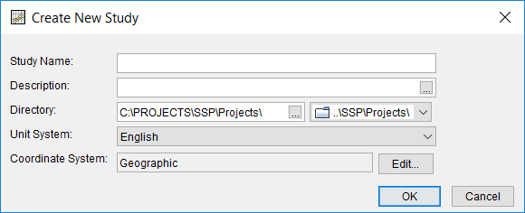
The user is required to enter a name for the study, select a directory to work in (a default location is provided), and select the desired units system. Adding a description of the study is optional. The user should also define a Coordinate System if background spatial data will be plotted. Multiple coordinate systems are provided for use. The choice of a coordinate system will not affect any computed results. Once you have entered all the information, press the OK button to have the information accepted. After the OK button is pressed, a subdirectory will be created under the user chosen directory. The subdirectory will be labeled with the same name as the user-entered study name. This study directory is where the HEC-SSP project file, as well as other study files and directories will be located. Additionally, a default map window will appear in the Main View Pane. However, the map window will be blank when it first opens.
Add a Background Map
By default, when you start a new project in HEC-SSP a default map window (called Base Map) will open in the Desktop window. Having a background map is optional in HEC-SSP. Not having a map will not prevent the user from importing and entering data, or performing an analysis and viewing results. The map is mostly a visual aid of the study area. Additionally, when you bring in gage data you can enter the map coordinates of the gage and it will be shown on the map. The user must supply a coordinate system other than X-Y (i.e. Geographic) for imported gage data to be displayed properly. Once a gage is located on the map you can right click on it to open a shortcut menu for viewing the data or graphing and tabulating the results.
To add a map layer to the default map, go to the Maps menu and select Add Map Layers. When this option is selected a file chooser window will appear, as shown in Figure 2, allowing the user to select map layers to bring into the map. The Create Copy option on the window will make a copy of the selected map and place it in the Maps subdirectory within the study folder.
Currently, the HEC-SSP software can load the following types of map layers: United States Geologic Survey (USGS) DLG, AutoCAD DXF, shapefile, Raster Image, USGS DEM, Arc Info DEM, ASCII NetTIN, Mr Sid, Open Street Maps, and Keyhole Markup Language (kml).
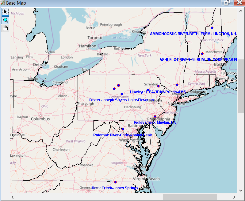
An example map is shown in Figure 3. This map contains a shapefile of state boundaries, data locations, and an internet map (open street map).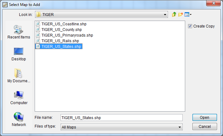
Import, Enter, and Edit Data
Before any analyses can be performed, the user must bring data into the HEC-SSP study. For a peak flow frequency analysis following guidelines in Bulletin 17C, the data must consist of an annual maximum series of streamflow. To bring data into HEC-SSP, go to the Data menu and select New. This will bring up the Data Importer as shown in Figure 4.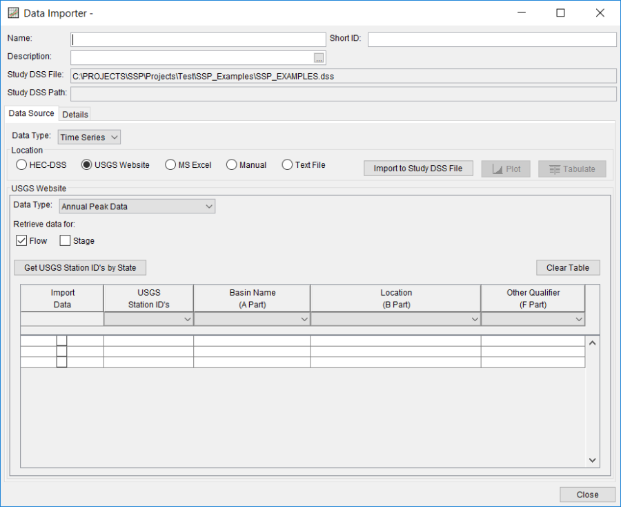
As shown in Figure 4, the Data Importer has fields for the Name, Short Identifier, and the Description of the data at the top of the window. Additionally, it lists the study DSS file name that the data will be stored in once it is brought into the study. The study DSS file is always labeled the same name as your study with the .dss file extension.
The Data Importer contains two tabs, Data Source and Details. The Data Source tab is shown first. This tab is used for selecting and defining a source for bringing data into the HEC-SSP study. Currently, there are five ways to bring data into an HEC-SSP study: import from another HEC-DSS file, import data from the USGS web site, import from a Microsoft Excel spreadsheet, manually enter the data into a table, and import the data from a text file. All of these methods will import data into the study DSS file.
For this example, importing data from the USGS website will be shown. For a complete description of the data importer see Chapter 4. To import data from the USGS website, first select the USGS Website option from the list of five options available in the Location panel. Next, select Annual Peak Data as the data type and make sure the Flow option is selected. The next step is to press the button labeled Get USGS Station ID's by State. When this button is pressed a window will appear (Figure 5) allowing the user to select a state from which to get data.
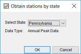
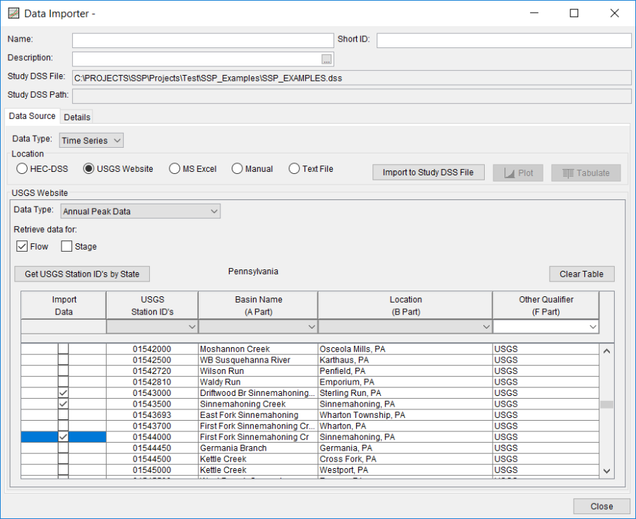
Once a state is selected, press the OK button and a list of the available gages from that state will appear in a pick list as shown in Figure 6. Check the boxes for all of the gages you would like to import and then press the Import to Study DSS File button. Once the import button is pressed, a process will begin during which the data will be downloaded from the USGS website and saved to the study DSS file. HEC-SSP will automatically name the data when importing multiple gages at one time. The USGS import process will download annual peak flow data, and the USGS data quality codes. The quality codes will be added as an addition object to the Data folder.
In addition to the data itself, any metadata that is available will be downloaded and stored with the data. The metadata can be viewed from the Details Tab on the Data Importer. Metadata can also be viewed or edited by opening the Metadata Editor. To open this editor, place the mouse on top of a data object in the Data folder and click the right mouse button. The shortcut menu contains an Edit Metadata option, as shown in Figure 7. The metadata editor is shown in Figure 8.
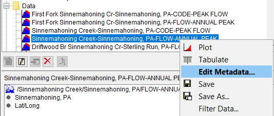
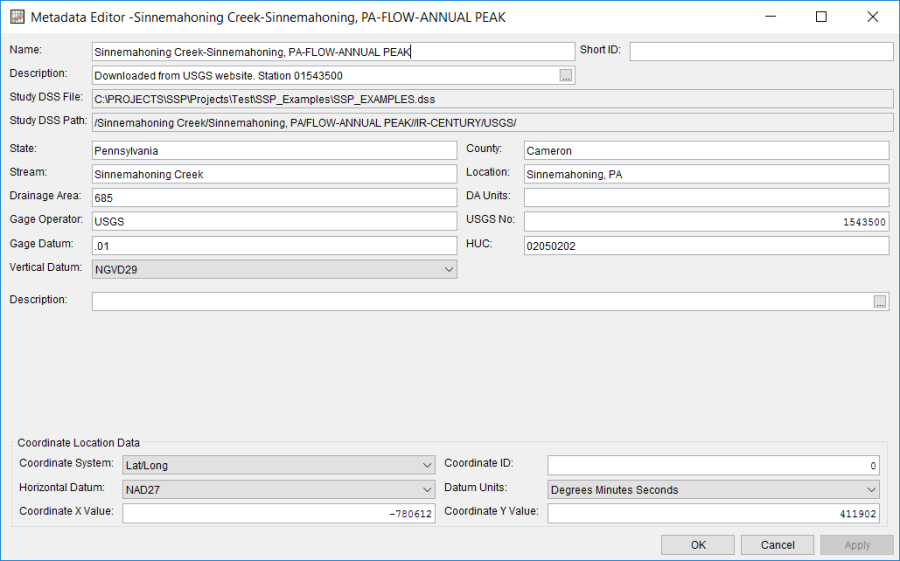
As shown in Figure 8, the metadata consists of the State, County, Stream, Location, Drainage Area, DA Units, Gage Operator, USGS Gage No., Gage Datum, HUC (Hydrologic Unit Code), Vertical Datum, and a description field. Additionally, the coordinate location of the data is shown. The coordinate location consists of Coordinate System, Coordinate ID, Horizontal Datum, Datum Units, Coordinate X Value, and Coordinate Y Value. Most of the USGS data is retrieved with the Latitude/Longitude coordinate system as shown in the example. In addition to editing the metadata, the Metadata Editor allows the user to change the name of the data, enter a short identifier, and enter a longer description.
If the metadata does not download automatically, the user has the option to enter any of the information by hand. Metadata will only be automatically generated when downloading data from the USGS website. Therefore, entering the metadata is required if the user wants it to be carried along with the study.
After the data is imported into the study, the user can select any one of the gages in the Data folder and Plot or Tabulate the data. The plot and tabulate options are available from the Data menu and from a shortcut menu that opens by clicking the right mouse button when the pointer is located on top of the gage object in the Data folder. If you select the Plot option, you will get a plot of the peak flow data for that gage. If you select the Tabulate option, you will get a table containing the data. Data values can be edited within the table; however, the editing mode must be turned on. To turn on editing, select the Edit | Allow Editing menu option. Use the File | Save or File | Save As menu option to save the data when you are satisfied with edits.
If the data has coordinate location information, it will then be plotted on top of the background maps. The software will convert the coordinates of the point data to the default coordinate system of the base map. The user can interact with the plotted points by right clicking on the gage icon in the map and a shortcut menu will appear as shown. The user has the option to edit the metadata, plot, tabulate, rename, or delete the data.
Performing the Flow Frequency Analysis
To perform a Bulletin 17 Analysis, go to the Analysis menu and select New | Bulletin 17 Flow Frequency. This will bring up an empty Bulletin 17 editor. As shown in Figure 9, the user must enter a name for the analysis, a description (optional), and select a flow data set (gage data stored in study DSS file). The DSS File Name and Report File are automatically filled in by the program. For now, the DSS File Name will be the study DSS file and the report file will have the same name as the analysis.
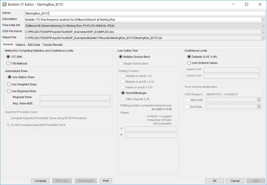
The editor window contains four tabs: General, Options, EMA Data, and Tabular Results. The General tab contains settings for Generalized Skew, Expected Probability Curve, Method for Computing Statistics and Confidence Limits, Plotting Positions, Confidence limits, a Time Window Modification, and Low Outlier Test. Default settings are already established for each of the options on the General tab; however, the user can change the default settings.
The Options tab contains information on Low Outlier Threshold, Historic Period Data (only used with Bulletin 17B procedures), and Output Frequency Ordinates. These options are not required for most analyses but may be necessary depending upon the data.
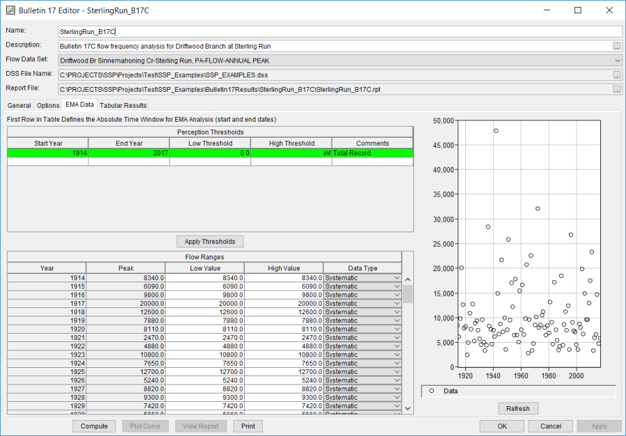
The EMA Data tab contains information specifically related to flow frequency analyses that make use of the procedures contained within Bulletin 17C, which uses the Expected Moments Algorithm (EMA) to compute flow frequency and confidence limits for the associated flow data set. A detailed description of each of the Bulletin 17C settings and options can be found in Chapter 5, Performing a Bulletin 17 Flow Frequency Analysis. The EMA Data tab is shown in Figure 10.
Once all of the settings and options have been selected, the user can click the Compute button to have the computations performed. When the computations have finished a message window will open stating Compute Complete. Press the OK button on the message window to close the window. Once the computations have finished the user can begin to look at output.
Viewing and Printing Results
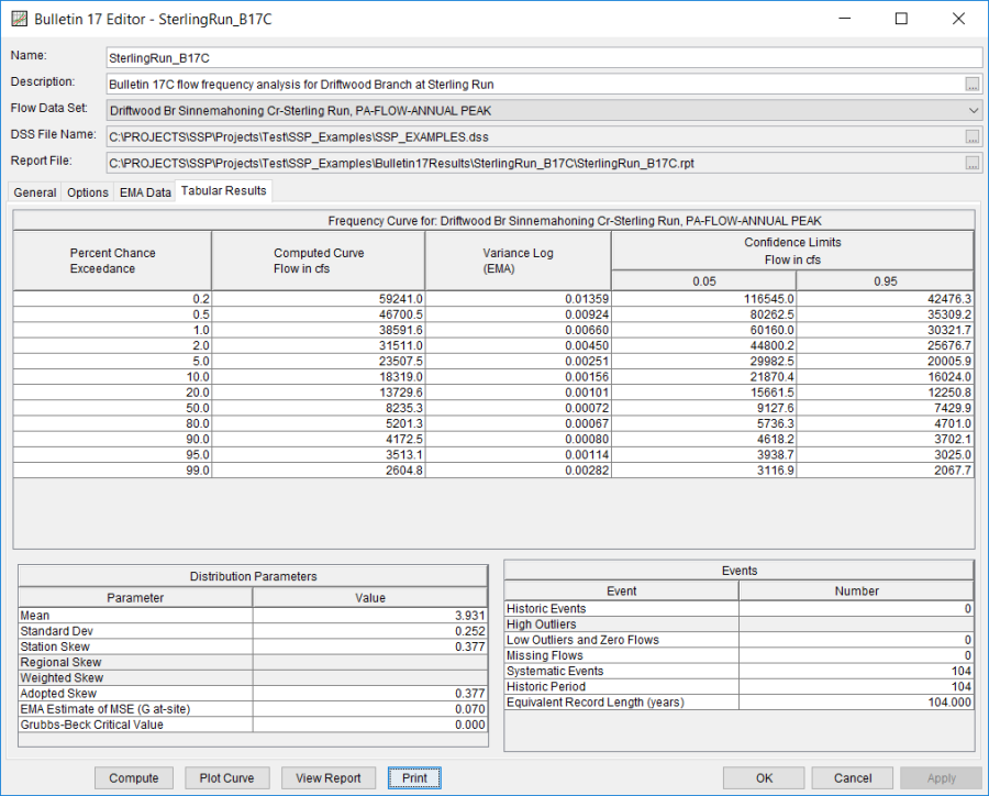
Tabular output can be viewed by selecting the Tabular Results tab. When this tab is pressed, a set of tables will appear as shown in Figure 11. The primary table on the Tabular Results tab consists of data for each frequency ordinate specified on the Options tab: the computed flow frequency (i.e. median) curve, the expected probability (i.e. mean) curve (if enabled on the General tab), variance (if using Bulletin 17C procedures), and the confidence limits for the two percentiles specified on the General tab. The second table (bottom left) contains parameters about the fitted Log Pearson Type III distribution, such as the mean, standard deviation, station skew, regional skew, weighted skew, and the adopted skew of the analysis. The third table (bottom right) contains the number of historic events, high outliers (if using Bulletin 17B procedures), low outliers and zero flows, missing flows, systematic events, the historic period, and the equivalent record length (if using Bulletin 17C procedures). The table can be sent to the printer by pressing the Print button at the bottom of the analysis window. The user can control the number of decimal digits shown in the result tables and in reports. Select Options from the Tools menu and then open the Results tab, as shown in Figure 11.
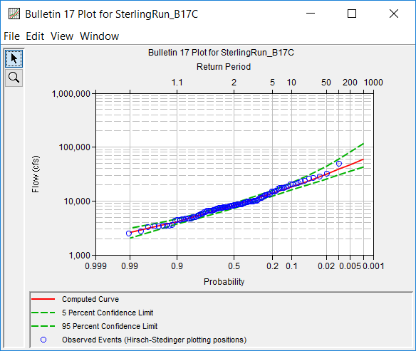
Graphical output can be obtained by pressing the Plot Curve button at the bottom of the analysis editor. When this button is pressed, a plot will appear like the one in Figure 12. This plot contains the computed frequency curve, the expected probability adjusted curve (if enabled on the General tab), the confidence limits, and the data points plotted using the plotting position method chosen on the General tab. Additionally, a plot title is listed at the top. The plot title is, by default, the user-defined name of the analysis. The user can modify the plot properties by selecting the Edit | Plot Properties menu option. A plot properties window will open that lets the user change the line style for each data type, change the axis labels, modify the plot title, and edit other plot properties. The user can also edit line styles by placing the mouse on top of the line or data point in the plot or legend and clicking the right mouse button and selecting Edit Properties. Individual curves can be highlighted by left clicking on an item within the legend. The plot can be printed or sent to the windows clipboard by using the Print and Copy to Clipboard options found under the File menu.
Marker lines and/or points can be added to a plot by placing the mouse anywhere in the plot area and clicking the right mouse button. Then select the Add Marker option to add a line or Add Marker Point to add a point. Draw properties can be edited for these user-defined lines and points by placing the mouse on top of the point or line and clicking the right mouse button. Then select the Edit Properties option in the shortcut menu.
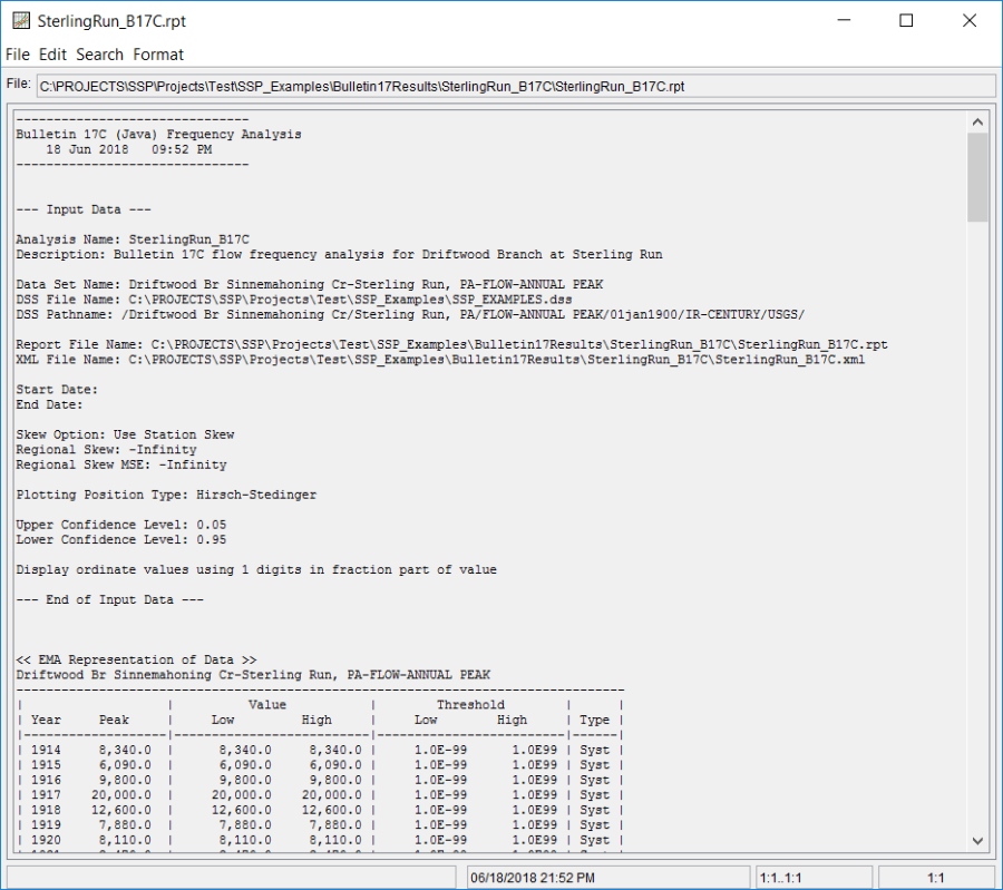
The final piece of output available from a flow frequency analysis is a text report file. The report file lists the user settings, the input data, plotting positions of the observed data, intermediate results, each of the various statistical tests performed (i.e. high and low outliers, historical data, etc.), and the final results. This file is often useful for understanding how the final frequency curve was computed. Press the View Report button at the bottom of the analysis editor to view the report file. When this button is pressed, a window will appear containing the report as shown in Figure 13. 