Task 4 Analyze Results from the Machine Learning Model
Results from the random forest models were evaluated in two ways. First, the random forest predicted HEC-HMS parameter adjustment factors were compared to factors that were set through manual calibration. Second, the random forest predicted HEC-HMS parameter adjustment factors were plugged into HEC-HMS model simulations and computed hydrographs were compared to observed streamflow.
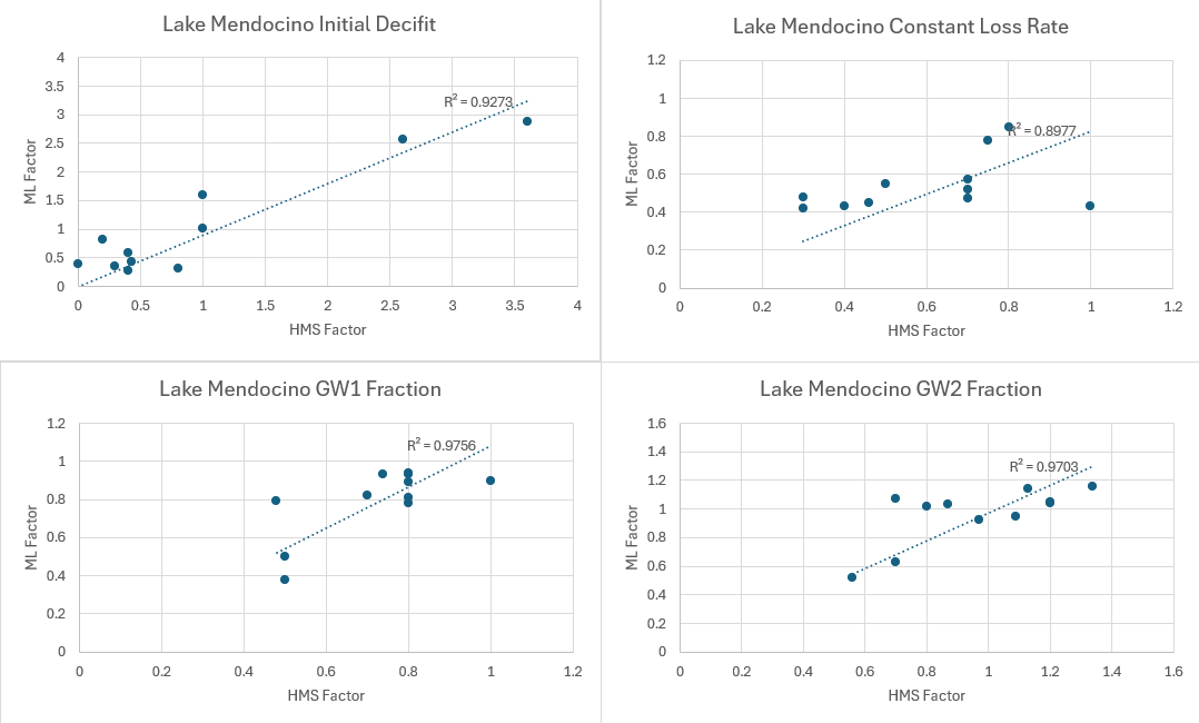
The Python script was configured to compute the simple linear R2 value (zero intercept) by comparing the random forest predicted HEC-HMS adjustment factors and those set through manual calibration. As shown in the table below, these values demonstrate good agreement in the predicted state variables and those set through manual calibration.
| Process and zone | R2 |
|---|---|
| Initial Baseflow Lake Mendocino Zone | 0.86102 |
| Initial Baseflow Hopland Zone | 0.98037 |
| Initial Baseflow Guerneville Zone | 0.95937 |
| Initial Baseflow Lake Sonoma Zone | 0.98926 |
| Initial Deficit Lake Mendocino Zone | 0.92718 |
| Initial Deficit Hopland Zone | 0.87681 |
| Initial Deficit Guerneville Zone | 0.929496 |
| Initial Deficit Lake Sonoma Zone | 0.880974 |
| Constant Loss Rate Lake Mendocino Zone | 0.902152 |
| Constant Loss Rate Hopland Zone | 0.853695 |
| Constant Loss Rate Guerneville Zone | 0.807263 |
| Constant Loss Rate Lake Sonoma Zone | 0.849145 |
| GW1 Fraction Lake Mendocino Zone | 0.975312 |
| GW1 Fraction Hopland Zone | 0.935556 |
| GW1 Fraction Guerneville Zone | 0.946215 |
| GW1 Fraction Lake Sonoma Zone | 0.958229 |
| GW2 Fraction Lake Mendocino Zone | 0.968632 |
| GW2 Fraction Hopland Zone | 0.94916 |
| GW2 Fraction Guerneville Zone | 0.961453 |
| GW2 Fraction Lake Sonoma Zone | 0.966991 |
The following figure show graphically what is in the R2 table above for the Calpella gage location. R2 values for the first ML model (one ML model for all HEC-HMS adjustment factors, SimpleMLScript_1.py) showed comparable performance. Significant improvement are not demonstrated by having a separate random forest model for each hydrologic process.

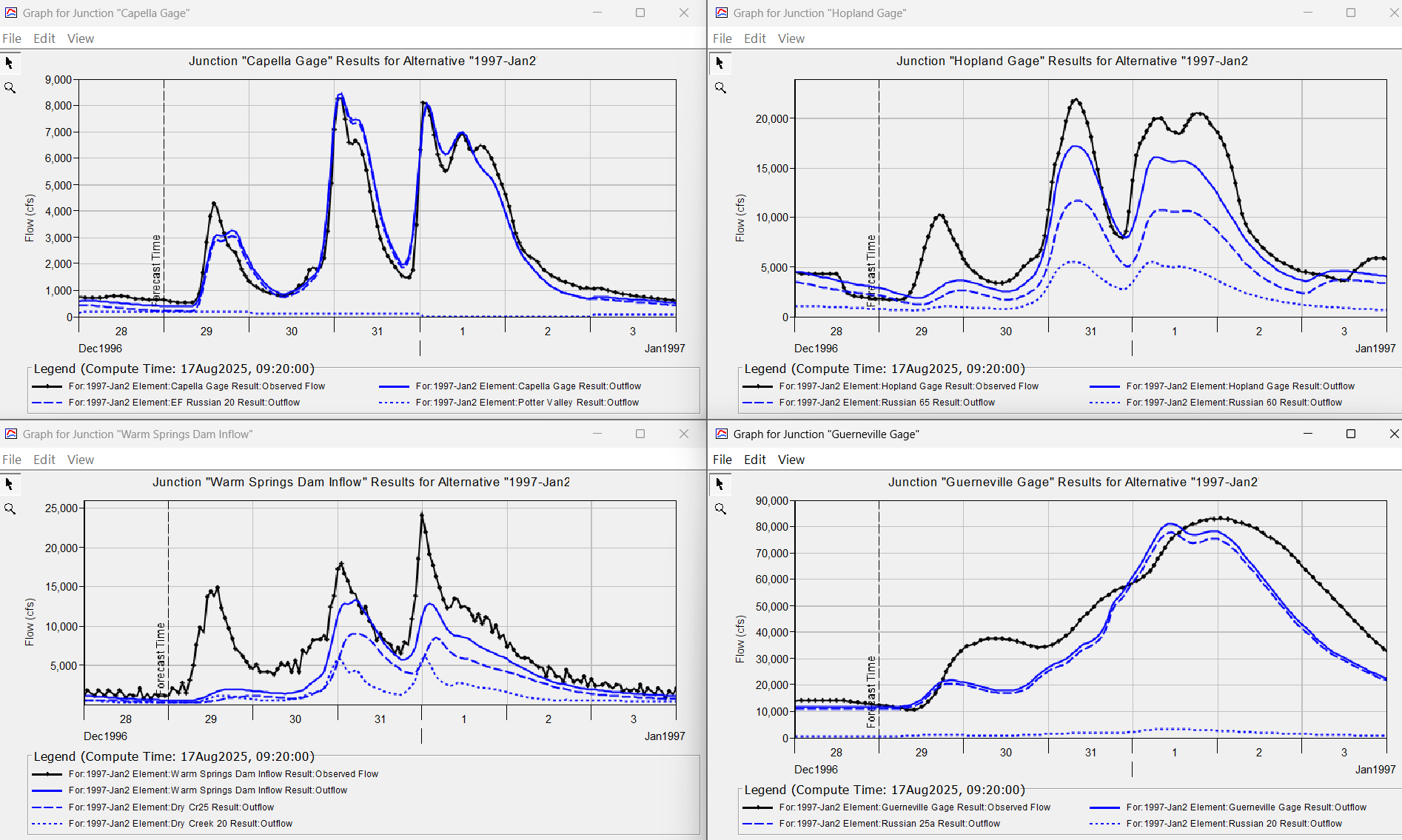
The following group of results show fairly good model performance at all four locations for the January 2, 1997 event. Starting a forecast simulation with the initial adjustment factors from the random forest model provides the modeler a great starting point that would only require slight modification to the initial deficit and constant loss rate adjustment factors for the Hopland, Guerneville, and Lake Sonoma Zones.

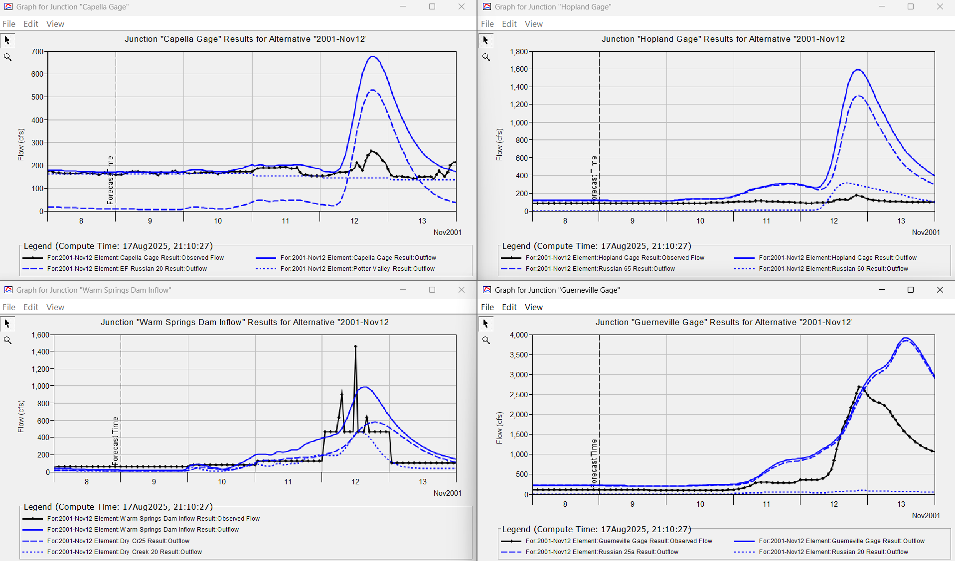
The following group of results DO NOT show good model performance at all four locations for the November, 11, 2001 event. However, the initial HEC-HMS adjustment factors set by the random forest models are fairly close to those found through manual calibration. The November, 11, 2001 storm was the first major storm of the season and the watershed was very dry when the storm began. The HEC-HMS adjustment factors estimate by the random forest models are much better than using average conditions to begin the calibration process.

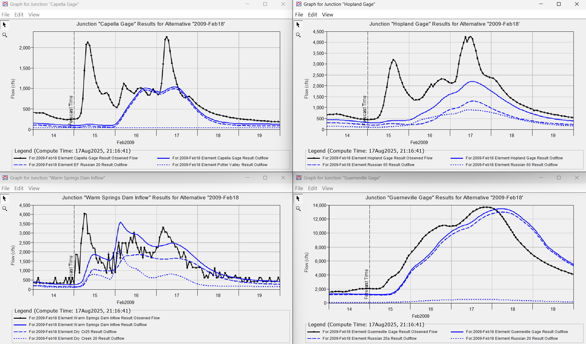
On the whole, the ML model predicted reasonable initial HEC-HMS adjustment factors for most events. Performance for the two February 2009 events was not as good as other events, results from the first event are shown in the following figure. January and February 2009 were drier than most years and the random forest model overpredicted the Initial Deficit adjustment factors. However, it would be relatively quick to manually set better adjustment factors after seeing the following results.

Conclusion
This example demonstrates a couple of key points:
- An HEC-HMS model can be quickly calibrated for real time flood forecasting by only adjusting a few model parameters that represent the initial state of the watershed. Even though the initial baseflow adjustment factor was modified for this example, reasonable results would have been seen by keeping a constant zonal override set for all events. This would have left only 4 adjustment factors to really change per event.
- The random forest models were able to assimilate past information, precipitation, temperature, and flow, and estimate reasonable initial HEC-HMS adjustment factors. In some cases the adjustment factors did not require further adjustment, the simulated hydrograph matched the observed hydrograph.
The random forest models took approximately 2 minutes to process the training data and fit the model and milliseconds to generate the predicted adjustment factors for the 11 test events. If applied to real-time forecasting, the random forest models would already exist and any time a new forecast created, it would automatically populate the starting HEC-HMS adjustment factors. Periodically, the random forest models would be updated as new events were added to the training dataset.