Using Machine Learning to Aid in Real-Time HEC-HMS Model Calibration
Application Data
Project Files
HEC-HMS 4.13 and Python 3.9.0 was used in this example.
- Russian_River_calibrated.zip - HEC-HMS project with 32 forecast simulations (these events are the "training" events), this model generated the adjustment factors to train the machine learning models.
- Predict.zip - 4 HEC-HMS projects, base, answer key, test 1 and test 2. The base project includes the 11 test events and a default set of adjustment factors defined (same adjustment factors for all 11 events). The answer key project has all 11 events manually calibrated using adjustment factors. The test 1 HEC-HMS project uses adjustment factors from the simple ML model (SimpleMLScript_1.py). The test 2 HEC-HMS project uses adjustment factors from ML models tuned to each process parameter (SimpleMLScript_2.py).
- Basin_Average.dss - DSS file with the precipitation and temperature predictor variables. Precipitation and temperature were averaged for the entire Russian River watershed.
- Flow time-series.dss - DSS file with the flow predictor variables.
- SimpleMLScript_1.py - ML script that uses 1 random forest model for all adjustment factors.
- SimpleMLScript_2.py - ML script that uses a separate random forest model for each type of adjustment factor; script also saves the linear R2 value.
Background
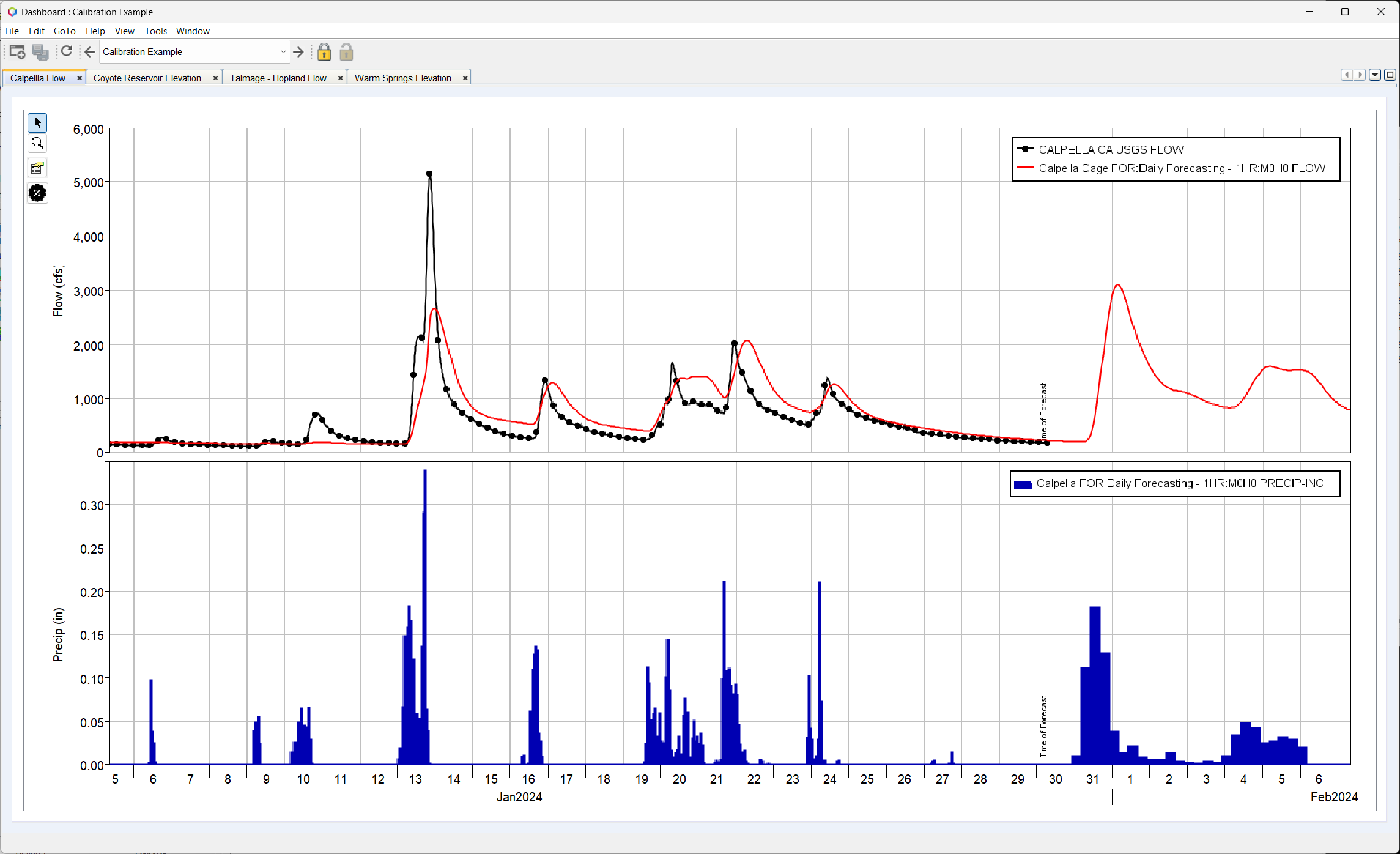
Reliable flow forecasts can be created by correctly setting the initial conditions for hydrologic processes in HEC-HMS. It can take significant time to "calibrate" a model by iterating to set the appropriate initial conditions. This is done by comparing the simulated and observed flow in the lookback period of a forecast and adjusting initial conditions. The figure below shows simulated and observed hydrographs, notice the model needs adjustment in the lookback period. This study/proposal looks at whether a machine learning algorithm can estimate initial state adjustment factors using preceding precipitation, temperature, and flow recorded before the event.

In many cases, only the initial states/conditions need to be appropriately set in order for the model to perform well. The unit hydrograph, baseflow, and reach routing parameters do not need to be adjusted when calibrating a model in real-time, assuming that the parameters have already been appropriately set. Typical model parameters that represent or are impacted by initial conditions included:
- Initial Baseflow
- Initial Moisture Deficit
- Constant Loss Rate
- This parameter is "estimated" using the saturated hydraulic conductivity; however, the conceptual infiltration model is rather simple and the constant loss rate could be tied to the moisture state in the watershed
- Linear Reservoir Baseflow GW 1 Fraction
- Linear Reservoir Baseflow GW 2 Fraction
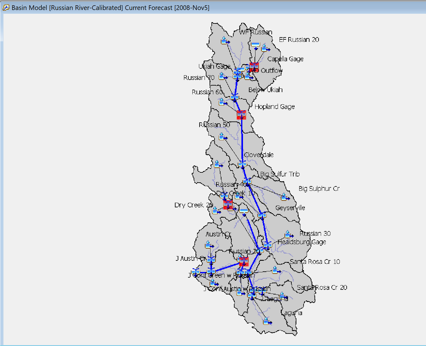
A slightly simplified HEC-HMS model of the Russian River watershed used in another example, HEC-HMS Model Calibration in CWMS, is used here. The HEC-HMS model used in this example was originally calibrated/validated to a 15 year continuous period of record. This model was used as the backbone for forecast alternatives that were set up to model discrete events within the period of record (water years 1995 - 2009). The figure below shows the spatial discretization of the watershed. There are four locations with observed flow, Lake Mendocino, Hopland, Guerneville, and Lake Sonoma.

Four zone were set up that included subbasins upstream of the locations with observed flow. The following figure shows the four zones.

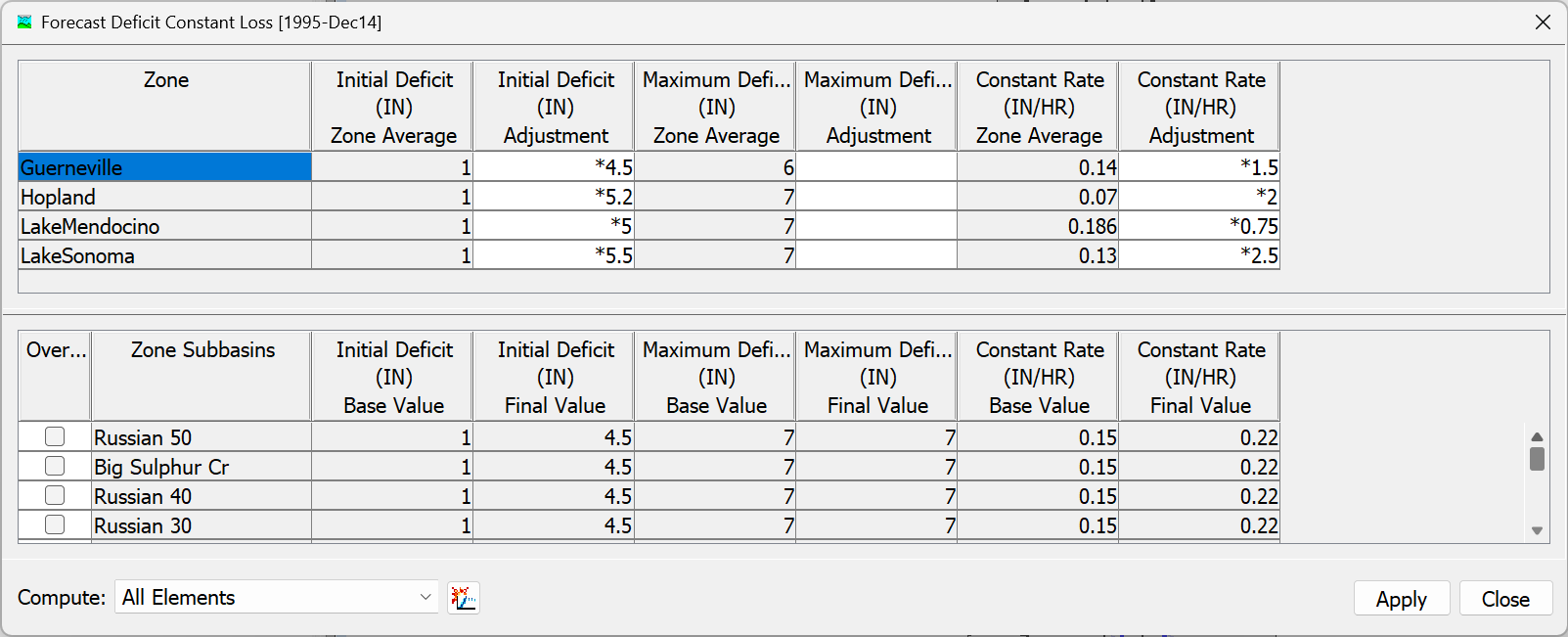
Within the forecast zonal editors, adjustment factors were used to modify the five parameters mentioned above to reflect initial states for the forecast simulations. The adjustment factors are applied to all subbasins in a zone. The following figure shows the adjustment factors applied to base (calibrated) parameters for the December 14, 1995 forecast. Notice the initial deficit has a base value of 1 inch and the adjustment factors are rather large, between 4.5 and 5.5. This large adjustment is needed because the watershed was still dry due to little rain in the summer and fall. The 120 day total rainfall prior to December 14, 1995 was 0.5 inches.

Objective
The purpose of this example is to demonstrate one approach to estimate initial state parameters in an HEC-HMS model when calibrating a model to real-time events. Being able to calibrate a model quickly is important, as water managers are often required to run multiple scenarios during flood events. They must accomplish these tasks quickly to provide enough time to disseminate and communicate model results within a reasonable time. Starting the calibration process with model parameters that are reasonable given the current conditions in the watershed will reduce the time needed to complete model calibration.
Tasks
Task 1 Develop the Datasets used to Train the Machine Learning Model
Task 2 Develop the Datasets used to Test the Machine Learning Model
Task 3 Train the Machine Learning Model and use it to Predict HEC-HMS Model Initial States
Task 4 Analyze Results from the Machine Learning Model