The Variable Type to use for simply reviewing results is the Computed Parameter type. Computed Parameter variables are available for all four elements types—Junction, Reservoir, Reach, and Diversion. Computed Parameter variables are not editable.
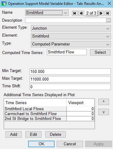
Figure: OSI Variable Editor—Configured for a Computed Parameter with Additional Time Series
The Operations Support Model Variable Editor will open next. Use this editor to specify the variable and identify any additional time-series that you want plotted with it. Start by selecting the Element Type.
Then, select the Element from the list of elements in your model.
Now, select Computed Parameter as your variable Type.
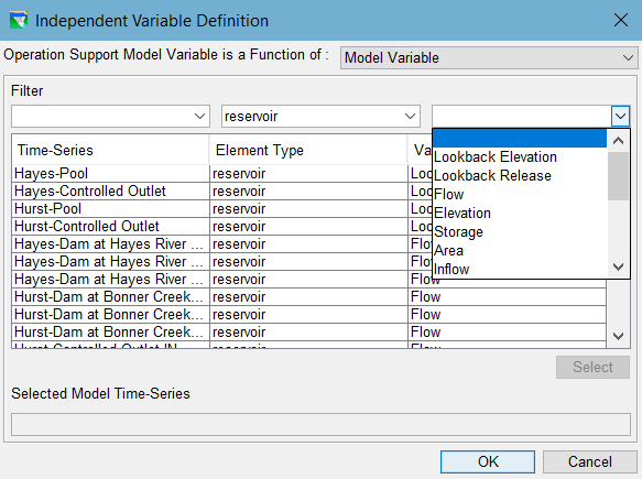
A field labeled Computed Time Series will appear below the Type field. Click the Select button to the right of this field.
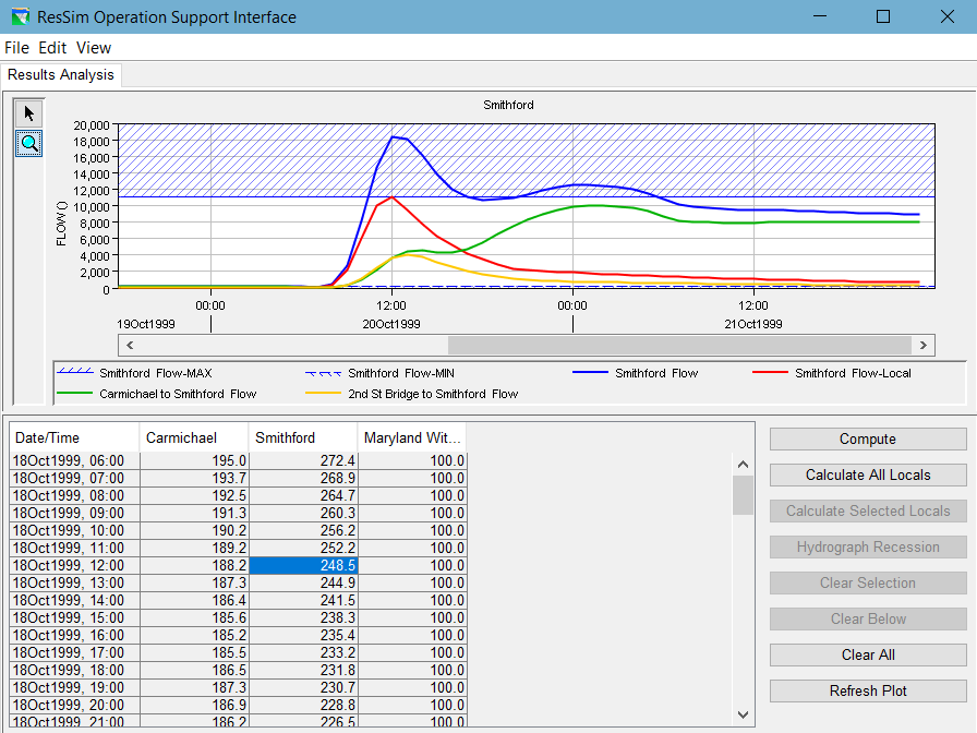
"Figure: OSI Example - Results Analysis Tab" shows the Results Analysis tab we assembled with the Smithford OSI Variable selected so that you can see how this variable is displayed. The Plot Panel shows a single plot window (viewport). In this plot window are curves for the Smithford flow as well as the other time series we chose to be plotted with it. In addition, the Minimum and Maximum limits that were specified for the variable are drawn with marker lines and a hatched fill. Since this variable is a computed parameter, it is not editable, so its data column in the Table Panel of the OSI is grey.
Figure: OSI Example - Results Analysis Tab
Although you might design a tab whose purpose is to simply display data for several variables (like we did in this example), you may find it useful to include a few Computed Parameter variables on the tabs you design for performing release overrides or computing incremental local flows. Look for Computed Parameter variables in the upcoming examples.