The Boundary Condition Set Editor (Figure 8.12) is designed to offer two options for entering the required input data for all boundary locations in a boundary condition set. The first option is to enter all the input data by boundary location using the view by location configuration (see Section 8.1.3). The second option is to enter the input data by WQ constituent, using the view by WQ constituent configuration (see Section 8.1.3). Either option opens the editable data panel. To add input data by location, for all required WQ constituents:
From the Boundary Condition Set Editor (Figure 8.12), from the boundary condition set navigation bar, select the set of interest (e.g., BoundaryConditionSet1 in Figure 8.12). Select the desired editor configuration by selecting either the Location or WQ Constituent radio button (Figure 8.12).
Select the location and WQ constituent of interest, and the editable data panel opens. For the example provided in Figure 8.12, the selected location and WQ constituent are Austin Ck Conf and Dissolved Oxygen, respectively.
Figure 8.12 – Boundary Condition Set Editor – Location Configuration – Enter Data Source – Atmospheric Pressure
From the editable data panel, specify the WQ constituent that is measured at the selected location (Figure 8.12). Sections 8.3.1 and 8.3.2 provide detailed instructions for entering and defining boundary conditions data. Once the data is entered in the editable data panel, a plot window opens at the bottom of the editable data panel, which displays the entered data.
The plot window has two options for viewing the entered data. The Plot Selected Data Source radio button (Figure 8.9) provides a plot of the entered data for only the currently selected Data Source.
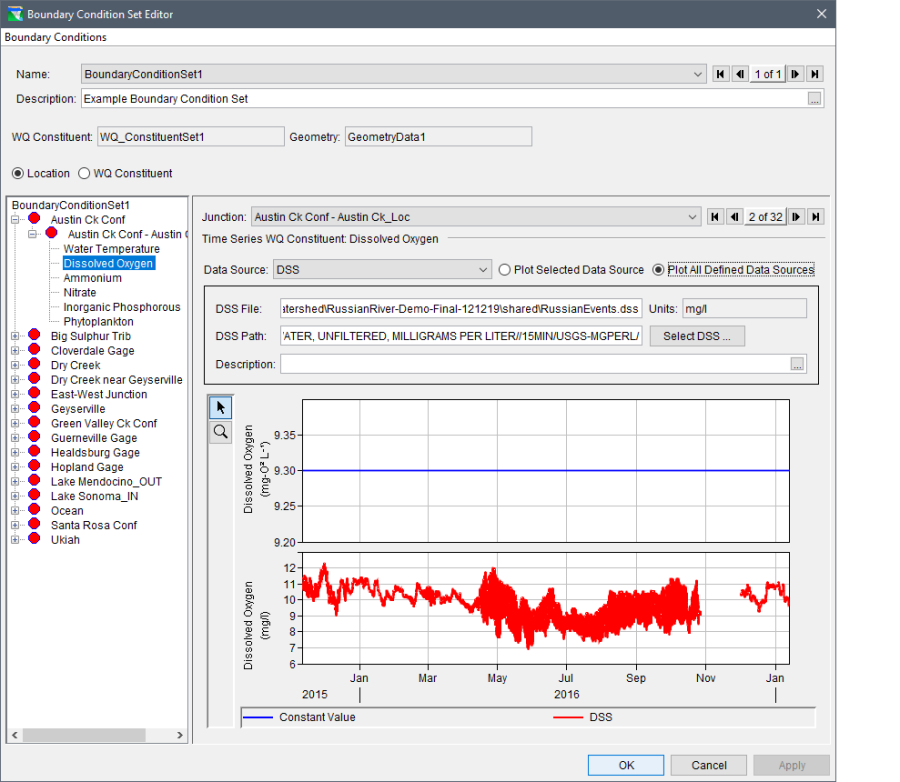
Alternatively, to view a plot containing all entered input data (entered from more than one data source option), select the Plot All Defined Data Sources radio button option to open a group plot (Figure 8.13). For the example provided in Figure 8.13, two plots display in the plot window for the data entered using the Constant Value and DSS data source options.
Note: The x-axis of the plot window changes depending on the Data Source and whether the Boundary Condition Set Editor is opened from the Water Quality module or the Simulation module (refer to Chapter 14). For example, if the plot contains DSS data, then the plot window displays the period of record (POR) for the selected HEC-DSS record when opened from the Water Quality module; however, if the Boundary Condition Set Editor is viewed in the Simulation module (refer to Chapter 14), then the plot window will use simulation time window.
Figure 8.13 – Boundary Condition Set Editor – Location Configuration – Plot All Defined Sources – Shortwave Radiation
The following sections provide instructions for entering data from each data source options and specifics for each of the required WQ constituents.