These methods examine pairs of grids and return geometric information such as the intersection or union of the extents.

GridUtilities.compatibleGrids

This method compares the coordinate system, cell size, and row and column positioning of two grids to determine if they are compatible for grid-to-grid operations. It returns the Boolean value true if the grids are compatible and false if they are not
Boolean GridUtilities.compatibleGrids(
GridData grid1,
GridData grid2)

This method may produce incorrect results for comparisons involving grids that use the SpecifiedGridInfo class for their GridInfo members. The flexibility that the SpecifiedGridInfo class provides for defining and labeling the coordinate system of a grid dramatically increases the complexity of comparing coordinate systems for equivalence. The method is coded to (we hope) minimize false returns when the grids are in fact compatible. In the future, a third-party library could be used to carry out coordinate system comparisons, which should produce more reliable results.

GridUtilities.intersectExtent

This method calculates the extent of the intersection of two compatible grids. The extent is returned as an array of four integers. If the grids are not compatible or do not intersect, all four values are set to zero.
int[] GridUtilities.intersectExtent (
GridData grid1,
GridData grid2)
The contents of the array (a) that the method returns are as follows:
a[0] = column number of origin cell
a[1] = row number of origin cell
a[2] = number of columns in the region (x extent)
a[3] = number of rows in the region (x extent)

GridUtilities.unionExtent

This method calculates the extent of the union of two compatible grids. The extent is returned as an array of four integers. If the grids are not compatible, all four values are set to zero.
int[] GridUtilities.intersectExtent (
GridData grid1,
GridData grid2)
The contents of the array (a) that the method returns are as follows:
a[0] = column number of origin cell
a[1] = row number of origin cell
a[2] = number of columns in the region (x extent)
a[3] = number of rows in the region (x extent)

Grids in DSS

Identifying Grid Records in DSS

Grid records in DSS are named according to a naming convention that differs slightly from the convention for time-series or paired-data records. Grids represent data over a region instead of at a single location and one grid record contains data for a single time interval or instantaneous value. The naming convention assigns the six pathname parts as follows.

• A-part: Refers to the grid reference system. At present, the HEC grid classes in Java support the HRAP and SHG grid systems grid systems as well as a UTM-based system that can be used outside the conterminous USA. For examples of grid A parts, see below. See appendices B, C and D for details of the grid systems.
• B-part: Contains the name of the region covered by the grid. For NEXRAD radar grids, this could be the name of the NWS River Forecast Center that produces the grid. For smaller grids produced by gageInterp or by extraction from RFC grids, this could be the name of a watershed.
• C-part: Refers to the parameter represented by the grid. Examples include PRECIP for precipitation, AIRTEMP for air temperature, SWE for snow-water equivalent, and ELEVATION for ground surface elevation. Refer to individual program manuals for conventions for parameter names.
• D-part: Contains the start time. This is the starting time of the interval covered by the grid. The date and time are given military-style (DDMMMYYYY for date and HHMM for time on a twenty-four hour clock) and the date and time are separated by a colon (. All times for grids should be given as UTC. Midnight is represented by 0000 if it is a starting time and 2400 if it is an ending time.
• E-part: Contains the end time. This is the ending time of the interval covered by the grid. The E part is blank for grids of instantaneous values.
• F-part: Refers to the version of the data. The version identifies the source of the data or otherwise distinguishes one set of grids from another. Version labels include STAGEIII for NWS stage III radar products, and INTERPOLATED for grids produced by GageInterp.

Example DSS grid pathnames:
The pathname below names an SHG precipitation grid for the Rogue River basin for the hour ending at 1900 UTC on May 3, 2003. The Rogue basin is in Oregon, so the grid represents the hour ending at noon local (Pacific Daylight) time. This grid was generated by GageInterp.
/SHG/ROGUE/PRECIP/03MAY2003:1800/03MAY2003:1900/GAGEINTERP/
The pathname below names a precipitation grid for the Missouri River basin for the hour ending at 0100 UTC. The grid comes from the Missouri Basin River Forecast Center, and is a product of the NWS's multi-sensor precipitation estimate.
/HRAP/MBRFC/PRECIP/22SEP2004:0000/22SEP2004:0100/MPE/
The pathname below names an HRAP grid representing a Quantitative Precipitation Forecast over the Ohio River Basin. This is a NWS product from the Ohio River RFC, and it covers the twenty-four hour period from noon June 1, 2001 to noon June 2, 2001 (UTC).
/HRAP/OHRFC/PRECIP/01JUN2001:1200/02JUN2001:1200/QPF/
The pathname below names an SHG temperature grid for the Rogue River basin. The cell size in this grid is 1000 meters instead of the default 2000 meters for SHG. Because the temperature is an instantaneous value at 0800, the E-part of the path is blank.
/SHG1K/ROGUE/AIRTEMP/22FEB2002:0800//GAGEINTERP/

Contents of a Grid Record in DSS

In HEC-DSS, both time-series and grid records consist of an array of sequential numerical values and an associated header describing the data in the array. In a time-series record, the value array represents the variation of a parameter's value through time at a fixed location. In a grid record, the value array represents the variation of a parameter's value through a range of locations (i.e., a region of the earth's surface) for a single interval of time. The header array of a grid record contains information about the parameter values (their units and some summary statistics) and the two-dimensional region that they represent (the number of rows and columns in the array, and the location of the grid in geo-referenced coordinates).
The contents of the grid header are described in section A.4 below for four types of grid records in DSS. The grid header types are:

• UNDEFINED—containing basic parameter and grid extent information, which is common to all grid types.
• HRAP—for US National Weather Service NEXRAD grids.
• Albers Equal-Area—including SHG grids.
• Specified Grid Info—a general-purpose grid type which contains a complete description of the Spatial Reference System (SRS) in which the grid's location is defined.

The HRAP and Albers grid headers contain additional descriptive information specific to those grid types. The Specified Grid Info header is potentially capable of describing grids in any coordinate system, including HRAP and SHG (Albers).

Storage of Grid Values

In the DSS file, grid parameter values are stored in a single array, starting with the value in the minimum-x, minimum-y (or lower left) cell in the two-dimensional array. The values proceed by row in increasing column numbers and increasing row numbers, as illustrated Below:

Two-Dimensional Grid

1One-Dimensional Array

f Parameter Values
The array of parameter values is always compressed before it is written to a DSS file. Two compression methods are used. One is a run-length encoding method, which replaces repeated zero and null values with the number of times zero or null was repeated. The second method is the deflate method, which is included in the zlib library described in RFC 1950. The deflate format itself is described in RFC 1951, and included in versions 1.1 and later of Java.

Grid Header Contents

Table A 1Grid Header Contents (All Types)
Notes:

• Info Flat Size should represent the size (in bytes) of the header of the grid record. This is implementation dependent and results may vary.
• Grid Type is the integer representation of the DSS record type of the grid. Grid types are numbered starting at 400, as follows.
  • 400: Unknown grid type. Grid Info contains only the common elements listed in table C.1a.
  • 410: HRAP grid type. Grid Info contains common elements and the HRAP data source. See table C.1b.
  • 420: Albers grid type. Grid Info contains common elements and Albers projection metadata. This is the type used for SHG grids. See table C.1b.
  • 430: Specified grid type. Grid Info contains common elements and additional metadata including a general-purpose definition of the spatial reference system. See table C.1c.
  • In some applications, a non-time-varying grid is indicated by adding 1 to the grid type. For example, 411 could be used as the grid type of an HRAP grid of some fixed property, such as ground elevation. To date, use of this convention has been inconsistent. Grid types ending in 1 can safely be assumed to be time-invariant, but grid types ending in 0 cannot always be assumed to be members of a sequence of time-varying grids.
• Start Time and End Time are represented by an integer number of minutes since 31 Dec 1899, 00:00. This number can be converted to an HecTime using the set() method.
• Data Units field can contain up to 12 ASCII characters.
• Data Type is one of the following.
  • 0 = Period Average
  • 1 = Period Cumulative
  • 2 = Instantaneous Value
  • 3 = Instantaneous Cumulative
  • 4 = Frequency
  • 5 = Invalid
• Lower Left Cell X and Y, and Number of Cells X and Y represent the row and column number of the origin, and the extent in rows and columns of the grid in the record, relative to the numbering system implied by the grid reference system (HRAP, SHG, etc.).
• Cell Size is a float value cast to an int data type for storage. It represents the size, in meters, of a cell in the grid. Cells are assumed to be square.
• Compression Method:
  • 0 = Undefined Compression Method
  • 101001 = Precip 2 Byte
  • 26 = Deflate using the ZLIB library function.
• Compressed Array Size is the number of bytes used in the DSS record to store the compressed array of grid values.
• Compression Scale Factor and Compression Base are values used for scaling the data in the array for storage. The base is subtracted from each value and the result is divided by the scale Factor. For precipitation in mm, the base is 0, and scale is 100, so that 5.00mm of rain is represented in the stored array as 500.
• Min Data Value, Max Data Value, and Mean Data Value apply to non-null values in the array, with their conventional meanings.
• Number of Ranges, Range Limit Table, and Range Counts provide a data summary. The range count array contains, in decreasing order, the counts of cells that are less than or equal to, the range limit values stored in the range limit array (stored in order of increasing value). The tables can contain up to 20 values. The default range array table contains 13 values (NULL, 0.0, 1E-7, 5.0, 10.0, 20.0, 50.0, 100.0, 200.0, 500.0, 1000.0, 2000.0, and 5000.0) which were set for precipitation values in mm for durations on the order of an hour. Other ranges limits can be set through the programming interface.

Table A 2Grid Header Contents (Fixed Spatial Reference)
Notes:

• Data Source field for HRAP headers can contain up to 12 ASCII characters
• Projection Datum for Albers headers is one of the following:
  • 0 = Undefined Projection Datum
  • 1 = NAD 27
  • 2 = NAD 83
• Projection Units field for Albers headers can contain up to 12 ASCII characters

Table A 3 Grid Header Contents (Specified Spatial Reference)
Notes:

• Version number is an integer. When a change in the stored information occurs the number will be increased. No dots or sub-versions will be used.
• The Length fields for SRS Name, SRS Definition, and Time Zone ID specify the number of integers used to store the Hollerith-encoded (four characters per int) SRS Name, SRS Definition, and Time Zone ID text fields.
• SRS Definition Type is one of the following:
  • 0 = Well-Known Text (WKT)
• Is Interval and Is Time-Stamped fields are stored as integers.
  • 0= False
  • 1 = True (any non-zero value will convert to True.)

All text fields in all GridInfo types are stored as Hollerith-encoded ASCII.

HRAP Grid System
The Hydrologic Rainfall Analysis Project (HRAP) grid is a square-celled map grid based on a Polar Stereographic map projection with the following parameters.
Units: Meters
Datum: Sphere (radius = 6371.2 km)
Standard Parallel: 60º 0' 0" North
Central Meridian: 105º 0' 0" West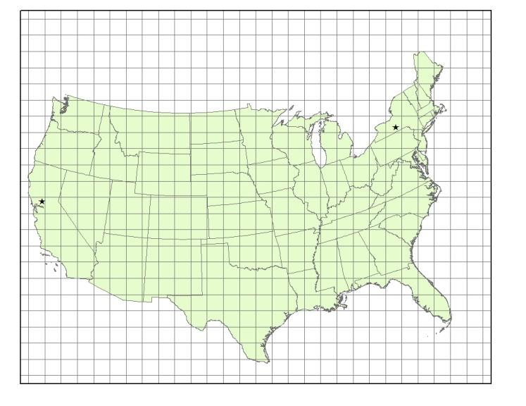
The mesh (cell) size of the grid is 4.7625 km, and the grid Y axis is aligned parallel with the central meridian (105 W). The grid is registered so that the North Pole lies exactly 400 cells in the positive X direction and 1600 cells in the positive Y direction from the grid origin. Equivalently, the lower left corner of cell number (401, 1601) is located at the North Pole.
Examples
As examples of cell identification in the HRAP system, indices of cells containing points in the western US and the eastern US are given.
Western United States: The location 121º 45′ west, 38º 35′ north (near Davis, California) projects to 260,174 m easting, 2,143,782 m northing, in the specified polar stereographic projection. In the HRAP system the indices of the cell containing this point are:
i = 54
j = 450
Eastern United States: The location 76º 30′ west, 42º 25′ north (near Ithaca, New York) projects to 4,410,804 m easting, 3,018,420 m northing, in the specified polar stereographic projection. In the HRAP system the indices of the cell containing this point are:
i = 926
j = 633

SHG Grid System
The standard hydrologic grid (SHG) is a variable-resolution square-celled map grid defined for the conterminous United States. The coordinate system of the grid is based on the Albers equal-area conic map projection with the following parameters.
Units: Meters
Datum: North American Datum, 1983 (NAD83)
1st Standard Parallel: 29º 30' 0" North
2nd Standard Parallel: 45º 30' 0" North
Central Meridian: 96º 0' 0" West
Latitude of Origin: 23º 0' 0" North
False Easting: 0.0
False Northing: 0.0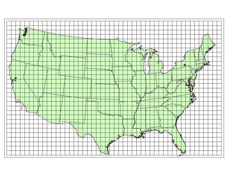
Users of the grid can select a resolution suitable for the scale and scope of the study for which it is being used. For general-purpose hydrologic modeling with NEXRAD radar precipitation data, HEC recommends 2000-meter cells, and HEC computer programs that use the SHG for calculation will select this cell size as a default. HEC will also support the following grid resolutions: 10,000-meter, 5,000-meter, 1,000-meter, 500-meter, 200-meter, 100-meter, fifty-meter, twenty-meter, ten-meter. The grids resulting from the different resolutions will be referred to as SHG two-kilometer, SHG one-kilometer, SHG 500-meter and so on. The corresponding DSS A-parts are SHG2K, SHG1K, SHG500, SHG100, SHG50, SHG20, and SHG10. A grid identified as SHG with no cell-size indication will be assumed to have two-kilometer cells.
For identification, each cell in the grid has a pair of integer indices (i, j) indicating the position, by cell count, of its southwest (or minimum-x, minimum-y) corner, relative to the grid's origin at 96°W, 23°N. For example the southwest corner of cell (121,346) in the SHG two-kilometer grid is located at an easting of 242000 meter and a northing of 692000 meter. To find the indices of the cell in which a point is located, find the point's easting and northing in the projected coordinate system defined above, and calculates the indices with the following formulas.
i = floor( easting / cellsize )
j = floor( northing / cellsize )
Where floor is the largest integer less than or equal to x.
Examples
As examples of cell identification in the SHG system, indices of cells containing points in the western US and the eastern US will be given in the one-kilometer, two-kilometer, and 500-meter SHG grids.
Western United States: The location 121º 45′ west, 38º 35′ north (near Davis, California) projects to -2195054 meter easting, 2027427 meter northing, in the specified Albers projection. In the SHG two-kilometer system the indices of the cell containing this point are:
i = floor( -2195054 / 2000 ) = floor( -1097.5 ) = -1098
j = floor( 2027427 / 2000 ) = floor( 1013.7 ) = 1013
Eastern United States: The location 76º 30′ west, 42º 25′ north (near Ithaca, New York) projects to 1583489 meter easting, 2320553 meter northing, in the specified Albers projection. In the SHG two-kilometer system the indices of the cell containing this point are:
i = floor(1583489 / 2000 ) = floor( 791.7 ) = 791
j = floor(2320553 / 2000 ) = floor( 1160.3) = 1160
In the SHG one-kilometer grid the indices are (1583, 2320), and in SHG 500-meter the indices are (3167, 4640).

Standardized UTM Grid System

The HRAP and SHG systems are undefined outside the conterminous US. To make practical applications of gridded computations in HEC-HMS outside of the CONUS region easier, HEC has developed a grid system based on UTM coordinates, using the cell-numbering conventions of SHG. By selecting a UTM zone (including the selection of northern or southern hemisphere) and cell size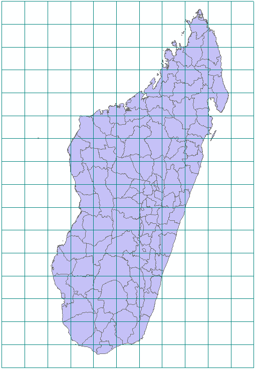

Units: Meters
Datum: World Geodetic System (WGS84)
Projected Coordinate System: Universal Transverse Mercator (UTM)
Zones: 1-60, North(N) or South(S)
(Example: Island of Madagascar, UTM 38S, cells are 100km square for illustration)


As with SHG, users of the grid can select a resolution suitable for the scale and scope of the study for which it is being used. HEC will support the following grid resolutions: 10,000-meter, 5,000-meter, 2,000-meter, 1,000-meter, 500-meter, 200-meter, 100-meter, fifty-meter, twenty-meter, ten-meter.
For identification, each cell in the grid has a pair of integer indices (i, j) indicating the position, by cell count, of its southwest (or minimum-x, minimum-y) corner, relative to the UTM zone coordinate origin. For example the southwest corner of cell (233, 4077) in a UTM two-kilometer grid is located at an easting of 466000 meters and a northing of 8154000 meters. To find the indices of the cell in which a point is located, find the point's easting and northing in the projected coordinate system defined above, and calculates the indices with the following formulas.

i = floor( easting / cellsize )
j = floor( northing / cellsize )
where floor is the largest integer less than or equal to x.




Examples
As examples of cell identification in a UTM spatial reference system, indices of cells containing points on the west and east coasts will be given in one-kilometer, two-kilometer, and 500-meter grids based on UTM zone 38S.
West coast: The location 43º 15′ 25" east, 22º 3′ 27" north (near the westernmost point of the island) projects to 320132 meters easting, 755978 meters northing, in the UTM zone 38 south. In a two-kilometer system the indices of the cell containing this point are:
i = floor( 320132/ 2000 ) = floor( 160.061 ) = 160
j = floor( 755978/ 2000 ) = floor( 377.989 ) = 377
East coast: The location 50º 31′ 49" east, 15º 20′ 11" south (near the easternmost point of the island) projects to 449580 meters easting, 8304412 meters northing, in UTM zone 38 south. In a two-kilometer system the indices of the cell containing this point are:
i = floor(449580/ 2000 ) = floor( 224.79) = 224
j = floor(8304412/ 2000 ) = floor(4152.206 ) = 4152

Note that a point at this longitude and latitude falls within the bounds of UTM zone 39 south. However, for this example it is assumed that one grid is being produced for precipitation over the whole island, so the coordinate are calculated for the easternmost zone (39 south) within the bounds of the grid.