Download PDF
Download page Boat Launch Analysis.
Boat Launch Analysis
Objective
You have been asked to advise what elevation a boat ramp should be built at Lake Oroville so that it gets the greatest use. Although Oroville is used all year long, the prime recreation months are April through October. The boat ramp should be at an elevation so that it will be used the greatest amount of time during that season. An additional constraint is that the ramp cannot have an elevation change greater than 50 feet.
In this task you will:
- Import USGS and CDEC data via import plugins
- Use CDEC storage and elevation data to generate a STOR-ELEV curve
- Use STOR-ELEV curve to convert USGS period of record data to elevation
- Perform Cyclic and Duration analyses on elevation data to solve the boat ramp problem
Task 1. Import Data
The California Data Exchange Center (CDEC) makes elevation, storage and inflow data available for Oroville Lake. However the full period of record is not available from CDEC.
Use the CDEC plugin to get both the storage, elevation and inflow data for Oroville for a portion of the period of record.
- Launch HEC-DSSVue; create a new DSS file named "Oroville.dss"
- Open the CDEC Import Plugin. Data >Import>CEDEC (Web).
- Start Date = Jan 01, 2006
- End Date = Today.
- The station name = "ORO".
- The duration code = "Daily",
- Sensor number for elevation, storage, and inflow are 6, 15 and 76 respectively.
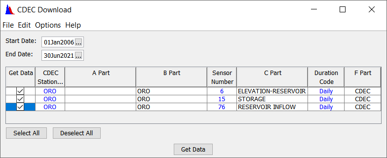
8. Select Get Data
9. Save this table so we can quickly re-import if need be; file>Save. This will save the Station Table to the user specified directory.
10. Name it "Oroville"
- The USGS also makes storage data available for Lake Oroville and has a more complete period of record than CDEC.
11. Get all available USGS data for lake Oroville
12. Open the USGS plugin from Data > Import >USGS Web
13. Select "Daily" for the Data Type
14. Check the "Retrieve Period of Record" box.
15. In the Station ID column enter 11406800 for the Oroville gage
16. Set the B-Part = "Oroville"
17. Set F-Part = "USGS"
18. Check the Import Data box.
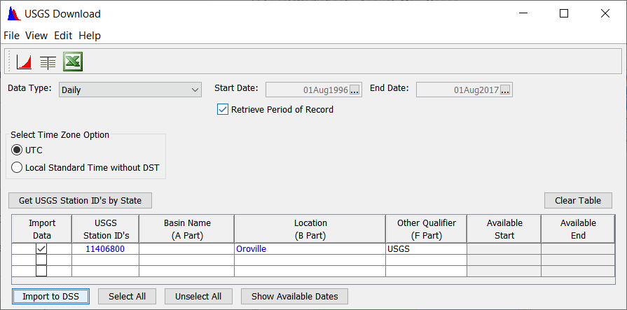
18. Select Import to DSS
19. Save this table so we can quickly re-import if need be, file>Save Station Table. Name it "Oroville"
20. Tabulate/Plot the new data
- If you hare having issues importing data, you can download the DSS data here: USGS&CDEC_DataIfNoInternet.dss
Question1. For the USGS data, what is the data type. What is the time frame? What are the units?
By tabulating the data we can see that the data type is period average and the units are "UNSPECIFIED". By plotting the data we can quickly see the time window of the data.
When importing data to DSS it is important to always scrutinize it before performing any analyses.
21. Clean up the newly imported storage data:
- Rename the record with a C-Part = "STORAGE" (Right-click>Rename)
- Set the units ="AF"
- Select the record and open Math Functions.
- In the General Tab select Set Units
The USGS gage has been recording data since the lake began to fill. This filling period might skew our duration and cyclic analyses for the boat ramp, so it needs to be removed:
22. Delete the filling period using the Graphical Editor (covered here). For consistency, lets delete all data prior to 1970.
We now have the period of record storage data for Oroville, and some elevation data. However, we need the full period of record elevation data for our analyses. In the next step we will generate a Storage-Elevation relationship to obtain elevation for the period of record.
Task 2. Generate Storage-Elevation relationship
Compute the storage-elevation curve:
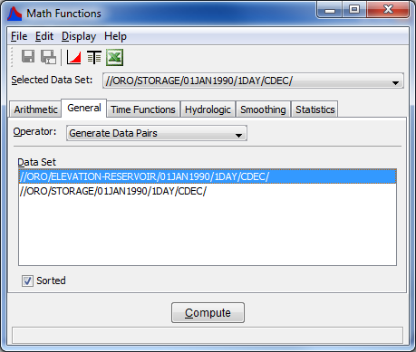
- Select the CDEC storage and elevation datasets you just retrieved by double-clicking them
- Open the Math Functions
- Select the "Generate Data Pairs" operator under the under the General tab.
- Use this function to compute a storage-elevation curve:
- The dataset in the drop down will be the "X" dataset, and the dataset highlighted below will be the "Y" dataset. Compute a storage elevation curve as shown below.
c. Plot your results to make sure you are happy with them.
d. Save the curve, using Save As, with a C-Part = STORAGE-ELEVATION
e. Close the Math Functions dialog
Now, do some clean up on this curve:
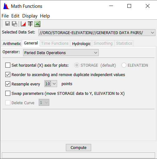
4. Clear all selected datasets and select the new Storage-Elevation Curve.
5. Open the Math Functions
6. Select the "Paired Data Operations" under the under the General tab.
7. Select the "Reorder to ascending and remove duplicate independent values",
8. Select resample every 10 points. Plot, verify and Save your new storage-elevation curve.
9. Close the math function editor
Task 3. Create POR Elevation Time Series
Compute an elevation time series from the USGS storage period of record:
- Clear all selections and select the USGS storage time series and your new storage-elevation curve.
- Open the Math Functions
- From the Hydrologic tab, choose the function "Rating Table".
- The dataset in the drop down should be the timeseries dataset, and the dataset highlighted below should be the rating table dataset.
- Press Compute
- Save your new data set with a C-Part of ELEV and F-Part of GENERATED
- Plot your new elevations.
We now have all the data required to perform our analysis
Task 4. Perform Analyses
First we will perform a Cyclic Analysis of elevation to became familiar how elevation varies throughout the season in Lake Oroville.
A cyclic analysis allows the user to create a set of pseudo time series that allow for easier investigation of data as well as inference of trends, and seasonality. Cyclic analyses can be performed within HEC-DSSVue using regular interval time series data (i.e. 1HOUR, 1DAY, 1MONTH). Time series that are produced by a cyclic analysis include maximum, minimum, average, standard deviation, 5-, 10-, 25-, 50-, 75-, 90-, and 95-percentile.
Perform a daily cyclic analysis on the data:
- Clear all selections and select the elevation data you generated.
- Open the math functions module.
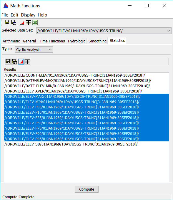
- select "cyclic analysis" in the Statistics tab of the math functions module
- Compute. The result datasets appear in the list in the bottom half of the editor.
- Select all of the non-exceedance percentile curves, and the min and max elevation curves as shown below and plot them. Note the results box has it's own plot button.
Question 2. What time of year is the reservoir the fullest? The emptiest?
The resrvoir is highest in the spring and the lowest in the fall and early winter. There have been a few big filling events in January and February as well.
Question 3. What are the max and min observed pool elevations?
Max = 902.5 Min = 628.6
Question 4. What else could you conclude from this data?
Without any prior knowledge about the reservoir, you can get an idea of the seasonality of the reservoirs operations. The filling period starts kicking off in January and the reservoir is evacuated in the fall. Elevation 900' appears to be an important upper limit and 648 appears to be an important lower limit. Can't conclude much about the hydrology of the watershed ...yet.
Now we will perform a duration analysis to determine how often our boat ramp will be usable. A duration curve estimates the likelihood that a daily stage or flow value will exceed a particular level. Duration curves are used when we need to know how often flow or stage is at or above a particular level. Common applications of a duration curve are:
6. Navigation: How often can we expect this channel to be navigable?
7. Run-of-river hydropower: How often can we expect to generate?
To perform a duration analysis:
8. Clear all selections, and select the elevation time series you created.
9. Open the Math Functions
10. From the Statistics tab, choose "Duration Analysis"
11. Choose the Bin Method, and a Duration Period of Other
12. In the Duration period table:
Pre Season 01JAN 01APR
Season 01APR 01NOV
Post Season 01NOV 01JAN
13. Delete the extra rows in the table by right-click> Delete Rows
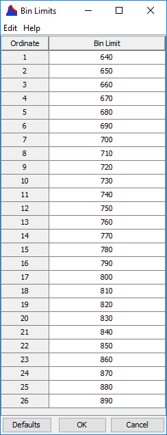
14. In the Bin area, select the User defined button and press the Set Limits button.
15. Change the table to have even elevations increments (e.g. every 10 feet starting at 640 and ending at 900). Click OK
16. After you set your bin limits, you will be prompted with another dialog to select Table Export option, press Cancel.
17. For plotting points, choose "ELEVATION on X Axis"
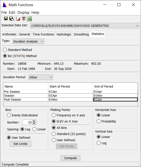
18. Press Compute,
19. Then tabulate your results.
Question 5. What do the values in this table represent?
The table shows the percent of time we can expect a certain elevation to be exceeded during each duration period.
Question 6. Using the results, if your boat ramp cannot have more than a 50' drop in elevation, at what elevation do you place bottom of the ramp so that it gets the most use during the recreation months of April through October?
A good way to think about this is to ask what percent of time is the boat ramp not usable. It is not usable when the elevation at the top of the ramp is exceeded. It is also not usable when the elevation at the bottom of the ramp is NOT exceeded.
Question 7. What elevation do you place the ramp for most use throughout the year?
Perform another duration analysis, but this time use an Annual Duration period.