Hydrologic Computations

With the lake levels and outflows screened and normalized to the same time scale, hourly reservoir inflow can be computed using the standard equation: 

where

S₂ and S₁ are the storages at the end and the beginning of the time period

$//<![CDATA[ \begin{array}{l}\Delta t\end{array} //]]>$ is the length of the time period

$//<![CDATA[ \begin{array}{l}\sum O\end{array} //]]>$ is the total outflow rate

$//<![CDATA[ \begin{array}{l}\sum I\end{array} //]]>$ is the net inflow

For this workshop, $//<![CDATA[ \begin{array}{l}\Delta t\end{array} //]]>$ equals 1 hour, or 3600 seconds.  The hourly average Lutz Park data provides the total outflow rate in cfs.  The only terms not already in hand are the top of the hour storages.  These will be calculated from hourly instantaneous reservoir levels using a storage-elevation relationship.  The reservoir levels are smoothed averages of the hourly levels at Fond Du Lac and Jefferson Park.

Task 1. Average Elevations

1. Clear any time window that may be set in HEC-DSSVue.

2. Select the following data sets:

   1. /LAKE WINNEBAGO/FOND DU LAC/ELEV/22Sep2000 - 31Oct2000/1Hour/COE-CST/

   2. /LAKE WINNEBAGO/JEFFERSON PARK/ELEV/22Sep2000 - 31Oct2000/1Hour/COE-CST/

3. launch the Math Functions dialog.

   

   If your Lake Winnebago/Jefferson Park did not translate the data from 2 after the hour and 2 after half pass the hour to being directly on the hour and half pass, please use the COE-CST-FIXED dataset instead of the COE-CST dataset.

4. Select Display → Original data with computed and Display → All Data Sets from the Math Functions menu bar.
5. Plot the data. 
   Note that the lake levels at the north and south ends fluctuate in opposite directions.  This ‘sloshing’ effect (seiche) occurs due to wind setup and atmospheric pressure differentials due to passing fronts.  The average of these two gages provides the best approximation of the still-water reservoir level needed for determining the storages.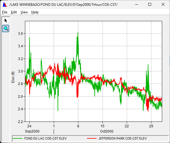
   
6. Close the plot.

7. Average the two elevations by adding the data sets together, then dividing the resultant by 2.  Be very careful with the mouse when stacking consecutive computations and start over if mistakes occur.  

8. Plot and tabulate the results.
   

9. Save your results using a B-part of MEAN LAKE
10. Exit the Math Functions dialog and close plots and tables.

Task 2. Smooth Elevations

Even though the mean levels provide a much closer approximation of the still-water reservoir level, wind-driven fluctuations still render them unsuitable for directly determining true reservoir storages.  Smoothing the levels with a moving-average technique dampens out the short-term fluctuations to provide a more realistic measure of storages changes.

1. Clear any time window and launch the Math Functions dialog with the data set named /LAKE WINNEBAGO/MEAN LAKE/ELEV/22Sep2000 - 31Oct2000/1Hour/COE-CST/
2. Smooth the elevation data using the Forward Moving Average, using 7 as the Number to Average Over.

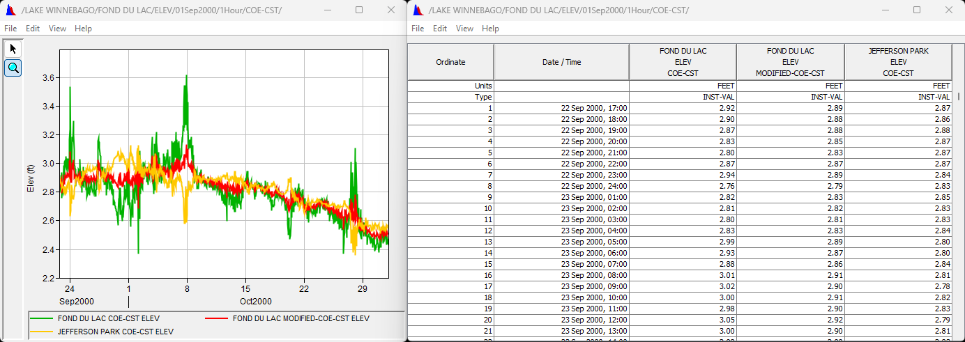
3. Plot the results. 
   You may have to zoom in and select the modified data in the legend to see the effects of the smoothing.
   The smoothed data set should generally track through the middle of the range of fluctuations. 
   

   Extra Credit: What are the pros and cons of using the various smoothing methods (described here)?

   Answer

   Smoothing Type	Pros	Cons
   Forward Moving Average	Values at the end of the time window (most recent data in real-time) are fully smoothed	Smoothed values lag in time. The smoother the result (averaging over more values), the greater the lag.
   Centered Moving Average	No lag of smoothed values as with Forward Moving Average	If not using reduced number of values at the beginning and end of the time widow are not in the smoothed data. If using reduced number of values at the beginning and end of the time window, those values are more poorly smoothed.
   Olympic Smoothing	Same as Centered Moving Average, but is more tolerant of spurious values	Same as Centered Moving Average

4. Save your results using a B part of SMOOTH MEAN LAKE
5. Close any plots or tables and exit the Math Functions dialog.

Task 3. Compute Storage

1. Clear any time window that may be set in HEC-DSSVue.

2. Select the following data sets:

   1. /LAKE WINNEBAGO/SMOOTH MEAN LAKE/ELEV/22Sep2000 - 31Oct2000/1Hour/COE-CST/
   2. /LAKE WINNEBAGO/MEAN LAKE/ELEV-STOR//1973/OSHKOSH DATUM/

3. launch the Math Functions dialog.

4. Compute reservoir storages using the Rating Table operator on the Hydrologic tab.

5. Tabulate and plot the results.
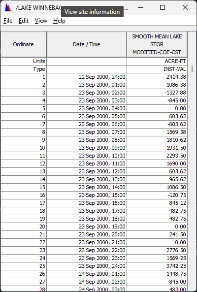
   Question 1. What are the units of the computed storages?

   Answer

   Acre-Ft

   

6. Save the storage results
   1. B part of SMOOTH MEAN LAKE
   2. C part of STOR
7. Exit the Math Functions dialog and close plots and tables.

Task 4. Compute Net Inflow

The DSS file now contains data sets for each of the terms needed to solve the equation for hourly net inflow.

1. Clear any time window that may be set in HEC-DSSVue.

2. Select the following data sets:

   1. /LAKE WINNEBAGO/SMOOTH MEAN LAKE/STOR/22Sep2000 - 31Oct2000/1Hour/COE-CST/
   2. /FOX RIVER/LUTZ PARK/FLOW-RES OUT/22Sep2000 - 31Oct2000/1Hour/USGS-CST-FIXED/

3. launch the Math Functions dialog.

4. Compute the change in reservoir storage for each hour. 
   Question 2. What function did you use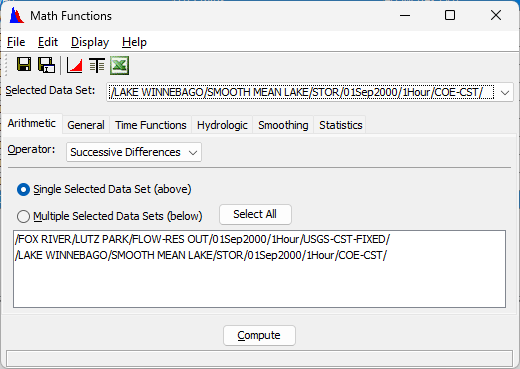?$//<![CDATA[ \begin{array}{l}\sum O\end{array} //]]>$

   Answer

   

5. Tabulate the results to see that the current data set consists of the storage change at the top of each hour.
   
   Question 3. What units are the values in?
   
   Answer

   ACRE-FT

   If we re-write our initial equation, as $//<![CDATA[ \begin{array}{l}\sum I = \frac{\Delta S}{\Delta t} +\sum O\end{array} //]]>$, we now have $//<![CDATA[ \begin{array}{l}\sum O\end{array} //]]>$,$//<![CDATA[ \begin{array}{l}\Delta S\end{array} //]]>$ for each interval, and $//<![CDATA[ \begin{array}{l}\Delta t\end{array} //]]>$ for each interval (the 1 hour interval of our data). The only thing remaining before we compute $//<![CDATA[ \begin{array}{l}\sum I\end{array} //]]>$, is to get our units straight.
   Question 4. What conversion factor do we need to convert $//<![CDATA[ \begin{array}{l}\frac{\Delta S}{\Delta t}\end{array} //]]>$ in acre-feet per hour to cfs?
   
   Answer

   $//<![CDATA[ \begin{array}{l}\LARGE \frac{acre \cdot ft}{hour} \vert \frac{43560 \cdot ft^2}{acre} \vert \frac{hour}{3600 \cdot s} = 12.1 \frac{ft^3}{s}\end{array} //]]>$

6. Using the General tab and Set Units operator, convert the storage changes from acre-ft/hour to cfs, using the conversion factor just computed.
   Question 5. Why is the method we just used (General/Set Units) preferable to using Arithmetic/Multiply or Arithmetic/Divide?
   
   Answer

   While using Multiply or Divide can be used to generate the same values, the Unit of the data will not be correct unless Set Units is subsequently used with a conversion factor of 1.0

7. Tabulate the results to see that the current data set consists of the storage change expressed as an hourly average inflow rate.
   
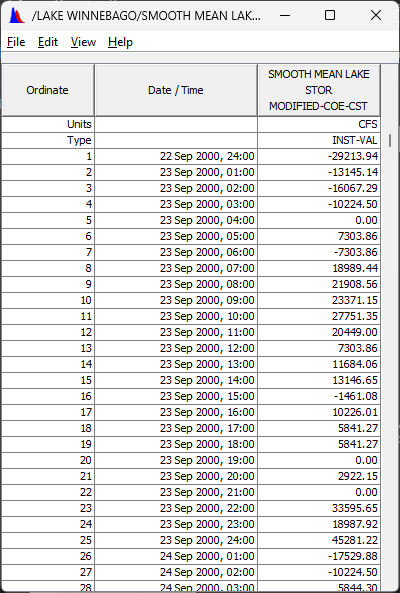
8. Save the result with a C part of STOR-CHANGE
9. Add the outflow to your storage changes.
10. Plot and Tabulate the results. 
    
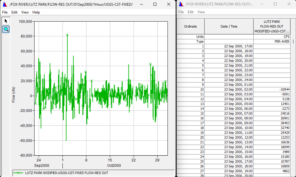
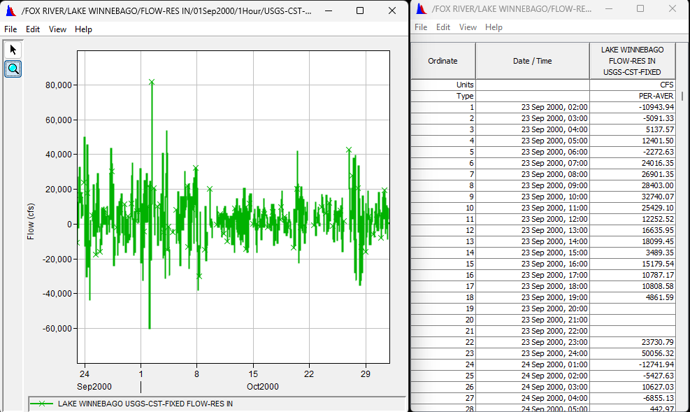
    The values should be positive and negative, with magnitudes in the tens of thousands.
11. Save this data set with a B part of LAKE WINNEBAGO and C part of FLOW-RES IN. 
12. Exit the Math Functions dialog.
13. Tabulate and plot the net inflow data to verify the numbers and units.