Hydrologic Functions
The Hydrologic tab (below) contains the following functions: Muskingum Routing, Straddle Stagger Routing, Modified Puls Routing, Rating Table, Reverse Rating Table, Two Variable Rating Table, Decaying Basin Wetness, Shift Adjustment, Period Constants, Multiple Linear Regression, Apply Multiple Linear Regression, Conic Interpolation, Polynomial, Polynomial with Integral, and Flow Accumulator Gage Processor.
Muskingum Routing
The Muskingum Routing function routes a regular interval time series data set by the Muskingum hydrologic routing method.
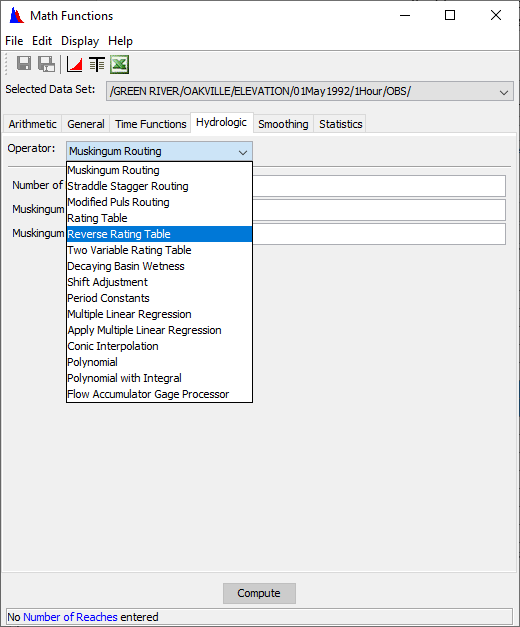
1. Choose the Hydrologic tab of the Math Functions screen and select the Muskingum Routing operator, as shown below.

2. From the Selected Data Set list, select the time series data set for routing.
3. In the Number of Reaches box, specify the number of routing subreaches.
4. In the Muskingum K box, enter the Muskingum "K" routing parameter (travel time, in hours).
5. In the Muskingum X box, enter the Muskingum "x" routing parameter. The Muskingum "x" value cannot be less than 0.0 (maximum attenuation) or greater than 0.5 (no attenuation).
6. Click Compute to route the selected time series data set.
An error message will be displayed if a compute is attempted using an invalid Muskingum "x" value, and no routing will be performed.
The set of Muskingum routing parameters entered may potentially produce numerical instabilities in the routed time series. The parameters are first checked by the function for possible instabilities before the routing proceeds. If instabilities are possible, a warning message box will appear presenting the details of the instabilities. Click the Yes button in the message box to proceed with the compute, or click No to cancel the operation.
Straddle Stagger Routing
The Straddle Stagger Routing function routes a regular interval time series data set by the Straddle Stagger hydrologic routing method.
To route a time series data set by the Straddle Stagger hydrologic routing method:
1.Choose the Hydrologic tab of the Math Functions screen and select the Straddle Stagger Routing operator, as shown below.

2. From the Selected Data Set list, select the time series data set for routing.
3. In the Number to Average box, enter the number of ordinates to average over (Straddle).
4. In the Number to Lag box, enter the number of ordinates to lag (Stagger).
5. In the Number of SubReaches box, enter the number of routing subreaches.
6. Click Compute to route the selected time series data set.
Modified Puls Routing
The Modified Puls Routing function routes a regular interval time series data set by the Modified Puls hydrologic routing method.
With the Modified Puls method, outflow from a routing reach is a unique function of storage. The storage-discharge relationship is entered into the function as a paired data set, where the x-values are storage and the y-values are discharge.
To route a time series data set by the Modified Puls hydrologic routing method:
1. Choose the Hydrologic tab of the Math Functions screen and select the Modified Puls Routing operator, as shown below. 
2. From the Selected Data Set list, select the time series data set for routing.
3. From the Storage-Discharge Paired Data Set list, select the paired data set containing the storage-discharge table. Only paired data sets will appear in this list, and only one data set at a time can be selected.
4. In the Number of SubReaches box, enter the number of routing subreaches.
5. In the Muskingum X box, enter the Muskingum "x" routing parameter. The Muskingum "x" value cannot be less than 0.0 or greater than 0.5. Enter 0.0 to route by the Modified Puls method, or a value greater than 0.0 to apply the Working R&D method.
6. Click Compute to route the selected time series data set.
Rating Table
The Rating Table function transforms/interpolates values in a time series data set using the rating table x-y values stored in a paired data set. For example, the Rating Table function can be used to transform stage values to flow values using a stage-flow rating table.
The units and parameter type of the resultant time series data set are duplicated from the y-units and y-parameter type of the rating table paired data set. For example, if a stage-flow rating table has a y-data parameter type of "FLOW" and y-units of "cfs", the resultant time series data set will have the data parameter type "FLOW" and the units "cfs".
To derive a new time series data set from the rating table interpolation based on the selected time series data set:
1. Choose the Hydrologic tab of the Math Functions screen and select the Rating Table operator, as shown below.

2. From the Selected Data Set list, select a time series data set for rating table interpolation. If the selected data set is not a time series, the remaining input boxes on the screen will be unavailable.
3. From the Rating Table list, select the paired data set containing the rating table information. Only paired data sets will appear in this list, and you may select only one data set at a time.
4. Click Compute to perform the rating table interpolation of the selected time series data set.
Reverse Rating Table
The Reverse Rating Table function transforms/interpolates values in a time series data set using the reverse of the rating table stored in a paired data set. For example, the Reverse Rating Table function can be used to transform flow values to stage values using a stage-flow rating table.
The units and parameter type of the resultant time series data set are duplicated from the x-units and x-parameter type of the rating table paired data set. For example, if a stage-flow rating table has an x-data parameter type of "STAGE" and x-units of "ft", the resultant time series data set will have the data parameter type "STAGE" and the units "ft".
To derive a new time series data set from the reverse rating table interpolation of the selected time series data set:
1. Choose the Hydrologic tab of the Math Functions screen and select the Reverse Rating Table operator, as shown below. 
2. From the Selected Data Set list, select a time series data set for reverse rating table interpolation. If the selected data set is not a time series, the remaining input boxes on the screen will be unavailable.
3. From the Rating Table list, select the paired data set containing the rating table information. Only paired data sets will appear in this list, and you may select only one data set at a time.
4. Click Compute to perform the reverse rating table interpolation of the selected time series data set.
Two Variable Rating Table
The Two Variable Rating Table function computes new time series values from the input of two other independent time series data sets. The functional relationship is specified by a table of values contained in a paired data set having multiple sets of x-y curves.
As an example, reservoir release is a function of both the gate opening height and reservoir elevation is shown below. 
Example of two variable rating table paired data, reservoir release as a function of reservoir elevation and gate opening height (curve labels).
For each gate opening height, there is a reservoir elevation-reservoir release curve, where reservoir elevation is the independent variable (x-values) and reservoir release is the dependent variable (y-values) of a paired data set. Each paired data curve has a curve label. In this case, the curve label is assigned the gate opening height. Using the paired data set shown in above, you may employ the Two Variable Rating Table function to interpolate time series values of reservoir elevation and gate opening height to develop a time series of reservoir release.
Times for the two input time series data sets must match. Curve labels must be set for curves in the rating table paired data set and must be interpretable as numeric values.
By default, the units and parameter type of the resultant time series data set are duplicated from the y-units and y-parameter type of the rating table paired data set.
The appearance of the Math Functions screen for the Two Variable Rating Table function is shown below.

Screen for Two Variable Rating Table Function
To derive a new time series data set from the two variable rating table interpolation of two other time series data sets:
1. Choose the Hydrologic tab of the Math Functions screen and select the Two Variable Rating Table operator.
2. From the Selected Data Set list, select the paired data set containing the rating table. If the selected data set is not a paired data set, the remaining input boxes on the screen will be unavailable.
3. From the two lists shown below the Data Set title, select the two input time series data sets.
■ Use the top list to select the time series data set matching the x-values parameter of the rating table. In the figure above, this is a time series data set of reservoir elevation.
■ Use the bottom list to select the time series data set matching the curve labels parameter. In the figure above this is a time series data set of gate opening height. You may select only one data set from a list.
4.Once the data sets are selected, click Compute to apply the Two Variable Rating Table function.
Decaying Basin Wetness
The Decaying Basin Wetness function computes a time series of decaying basin wetness parameters from a regular interval time series data set of incremental precipitation by:
TSPar(t) = Rate * TSPar(t-1) + TSPrecip(t)
where Rate is the decay rate and 0 < Rate < 1.
The first value of the resultant time series, TSPar(1), is set to the first value in the precipitation time series, TSPrecip (1). Missing values in the precipitation time series are zero for the above computation.
To compute a time series of decaying basin wetness parameters:
1. Choose the Hydrologic tab of the Math Functions screen and select the Decaying Basin Wetness operator, as shown below.

2. From the Selected Data Set list, select the time series data set of incremental precipitation.
3. Enter the Decay Rate. This value must be greater than 0.0 and less than 1.0.
4. Click Compute.
Shift Adjustment
The Shift Adjustment function linearly interpolates values in the primary time series data set to the times defined by a second time series data set. If times in the new time series precede the first data point in the primary time series, the value for these times is set to 0.0. If times in the new time series occur after the last data point in the primary time series, the value for these times is set to the value of the last point in the primary time series. Interpolation of values with the Shift Adjustment function is shown below.

Interpolation of Time Series Values using Shift Adjustment Function
Both time series data sets may be regular or irregular interval. Interpolated points must be bracketed or coincident with valid (not missing) values in the original time series; otherwise the values are set as missing.
To generate a new time series of shift adjustments:
1.Choose the Hydrologic tab of the Math Functions screen and select the Shift Adjustment operator, as shown below.

2. From the Selected Data Set list, select the primary time series data set. This data set has the values for the interpolation.
3. From the Data Set for time pattern list, which is located in the bottom part of the window, select the second time series data set. This data set has the times for the interpolation.
4. Click Compute.
Period Constants
The Period Constants function applies values in the primary time series data set to the times defined by a second time series data set. Both time series data sets may be regular or irregular interval. Values in the new time series are set according to:
ts1(j) ≤ tsnew(i) < ts1(j+1) , TSNEW(i) = TS1(j)
where ts1 is the time in the primary time series, TS1 is the value in the primary time series, tsnew is the time in the new time series, TSNEW is the value in the new time series.
If times in the new time series precede the first data point in the primary time series, the value for these times is set to missing. If times in the new time series occur after the last data point in the primary time series, the value for these times is set to the value of the last point in the primary time series. Interpolation of values with the Period Constants function is shown below.

Interpolation of Time Series Values using Period Constants Function
To generate a new time series of period constants:
1. Choose the Hydrologic tab of the Math Functions screen and select the Period Constants operator.
2. From the Selected Data Set list, select the primary time series data set. This data set has the values for the interpolation.
3. From the Data Set for time pattern list, which is located in the bottom part of the window, select the second time series data set. This data set has the times for the interpolation.
4. Click Compute.
Multiple Linear Regression
The Multiple Linear Regression function computes the multiple linear regression coefficients between a primary time series data set and a collection of independent time series data sets, and stores the regression coefficients in a new paired data set. This paired data set may be used with the Apply Multiple Linear Regression function, in the next section, to derive a new estimated time series.
For the general linear regression equation, a dependent variable, Y, may be computed from a set independent variables, Xn:
Y = B0 + B1*X1 + B2*X2 + B3*X3
where Bn are the linear regression coefficients.
For time series data, an estimate of the primary time series values may be computed from a set of independent time series data sets using regression coefficients such that:
TsEstimate(t) = B0 + B1*TS1(t) + B2*TS2(t) + … + Bn*TSn(t)
where Bn are the set of regression coefficients and TSn are the time series data sets.
All the time series data sets must be regular interval and have the same time interval. The function filters the data to determine the time period common to all data sets and uses only those points in the regression analysis. For any given time, if a value is missing in any time series, no data for that time is processed. Optional minimum and maximum limits can be set to exclude values in the primary time series which fall outside a specified range.
To compute the set of multiple linear regression coefficients:
1. Choose the Hydrologic tab of the Math Functions screen and select the Multiple Linear Regression operator.

2. From the Selected Data Set list, select primary time series data set. If the selected data set is not a time series data set, the remaining input boxes on the screen are unavailable.
3. From the Independent Time Series Data Sets list, select one or more of the independent time series data sets (by clicking, control-click or shift-click).
4. Click Compute to derive new a paired data set containing the linear regression coefficients.

Apply Multiple Linear Regression
The Apply Multiple Linear Regression function applies the multiple linear regression coefficients computed with the Multiple Linear Regression function (see the previous section). The coefficients, stored in a paired data set, are applied to a collection of independent time series data sets to derive a new estimated time series data set.
For time series data, an estimate of the primary time series values may be computed from a set of independent time series data sets using regression coefficients such that:
Y = B0 + B1*X1 + B2*X2 + B3*X3
where Bn are the linear regression coefficients.
For time series data, an estimate of the original time series values may be computed from a set of independent time series data using regression coefficients such that:
TsEstimate(t) = B0 + B1*TS1(t) + B2*TS2(t) + … + Bn*TSn(t)
where Bn are the set of regression coefficients and TSn are the time series data sets.
The number regression coefficients in the paired data set must be one more than the number of independent time series data sets. The collection of selected time series data sets should be in the same order as when the regression coefficients were computed. The displayed list of time series is sorted alphabetically in the dialog. The user should be aware if the names of the time series data sets used for coefficient generation are substantially different from the data names used in this function.
All the time series data sets must be regular interval and have the same time interval. The function filters the data to determine the time period common to all time series data sets and uses only those points in the regression analysis. For any given time, if a value is missing in any time series, the value in the resultant time series is set to missing. You can also set optional minimum and maximum value limits. Computed values in the resultant time series, which fall outside the specified range, are set to missing.
Names, parameter type and unit labels for the resultant time series data set are taken from the first time series data set. The "F part" (Version) in the new data set is set to "COMPUTED."
To apply a set of multiple linear regression coefficients to derive a new time series data set:
1. Choose the Hydrologic tab of the Math Functions screen and select the Apply Multiple Linear Regression operator, as shown below.

2. From the Selected Data Set list, select the paired data set containing the regression coefficients. If the selected data set is not a paired data set, the remaining input boxes on the screen are unavailable.
3. From the Independent Time Series Data Sets list, select one or more of the independent time series data sets. (You can select a single data set by clicking on it; select multiple contiguous data sets using Shift+Click, or select multiple, non-contiguous data sets using Ctrl+Click.)
4.Click Compute.
Conic Interpolation
The Conic Interpolation function transforms values in a time series data set by conic interpolation using an elevation-area table stored in a paired data set. The first value pair in the paired data set contains the initial conic depth and the initial storage volume at the first elevation (given in the next value pair). If the initial conic depth is missing, one is computed by the function. Values in the elevation-area table are stored in ascending order.
The Conic Interpolation function can interpolate a time series of elevation to derive a time series of storage or area. The function can interpolate a time series of storage to derive a time series of elevation or area. If the output time series is elevation, the output units are assigned from the x-units of the paired data set. If the output time series is area, the output units are assigned from the y-units of the paired data set. If the output time series is storage, the output units are undefined.
The appearance of the Math Functions screen for the Conic Interpolation function is shown below. The Conic Interpolation function is accessed from the Hydrologic tab of the Math Functions screen.

To perform the conic interpolation of a of elevation or storage:
1.Choose the Hydrologic tab of the Math Functions screen and select the Conic Interpolation operator.
2.From the Selected Data Set list, select a time series data set. If the selected data set is not a time series, the remaining input boxes on the screen are unavailable.
3. From the Conic Interpolation Table list, select the paired data set containing the conic interpolation table. Only paired data sets will appear in this list, and only one data set at a time can be selected.
4. From the Input Type list, select the parameter type of the input time series data (Elevation or Storage).
5. From the Output Type list, select the desired output data type (Storage, Elevation or Area).
6. In the Storage Scale box, enter factor for the scale of the storage output values. By default this value is 1. The value is used to scale input (by multiplying) and output (by dividing) storage values. For example, if the area in the conic interpolation table is expressed in sq. ft., the storage scale could be set to 43560 to convert the storage output to acre-ft.
7. Click Compute to interpolate the selected time series data set.
Polynomial
The Polynomial function computes a polynomial transform of a regular or irregular interval time series data using the polynomial coefficients in a paired data set. Missing values in the input time series data remain missing in the resultant time series data set.
A new time series can be computed from an existing time series with the polynomial expression,
TS2 (t) = B1* TS1(t) + B2* TS1(t) 2 + ... + Bn* TS1(t) n
where Bn are the polynomial coefficients for term "n."
Values for the polynomial coefficients are stored in the x-values of a paired data set. Before the above equation is applied, values in the input time series are adjusted by subtracting off the paired data "datum" value if defined. The x-units and parameter type from the paired data set are applied to the resultant time series data set.
To compute the polynomial transform of a selected time series data set:
1. Choose the Hydrologic tab of the Math Functions screen and select the Polynomial operator.
2. From the Selected Data Set list, select a time series data set. If the selected data set is not a time series, the remaining input boxes on the screen will be unavailable.
3. From the Polynomial Coefficients list, select the paired data set containing the polynomial coefficients. Only paired data sets will appear in this list, and you may select only one data set at a time.
4. Click Compute to perform the polynomial transform of the selected time series data set.
Polynomial with Integral
The Polynomial with Integral function computes a polynomial transform with integral of a regular or irregular interval time series data using the polynomial coefficients in a paired data set. Missing values in the input time series data remain missing in the resultant time series data set.
The polynomial transform coefficients are integrated, with the new time series values computed from an existing time series by the expression,
TS2 (t) = B1* TS1(t) 2/2 + B2*TS1(t)3/3+ ... + Bn* TS1(t) n+1/(n+1)
where Bn are the polynomial coefficients for term "n".
Values for the polynomial coefficients are stored in the x-values of a paired data set. Before the above equation is applied, values in the input time series are adjusted by subtracting off the paired data "datum" value if defined. The x-units and parameter type from the paired data set are applied to the resultant time series data set.
To compute the polynomial transform with integral of a selected time series data set:
1. Choose the Hydrologic tab of the Math Functions screen and select the Polynomial with Integral operator.
2. From the Selected Data Set list, select a time series data set. If the selected data set is not a time series, the remaining input boxes on the screen will be unavailable.
3. From the Polynomial Coefficients list, select the paired data set containing the polynomial coefficients. Only paired data sets will appear in this list, and you may select only one data set at a time.
4.Click Compute.
Flow Accumulator Gage Processor
The Flow Accumulator Gage Processor function computes the time series period-average flows from a flow accumulator type gage. Accumulator gage data consists of time series data sets of accumulated flow and counts. The two input time series data sets must match times exactly.
A new time series data set is derived from the time series of flow and counts by:
TsNew(t) = (TsAccFlow(t) - TsAccFlow(t-1)) / (TsCount(t) - TsCount(t-1))
where TsAccFlow is the gage accumulated flow time series and TsCount is the gage time series of counts.
In the above equation, if TsAccFlow(t), TsAccFlow(t-1), TsCount(t) or TsCount(t-1) are missing, TsNew(t) is set to missing. The new time series is assigned the data type "PER-AVER".
To process the flow accumulator type data:
1. Choose the Hydrologic tab of the Math Functions screen and select the Flow Accumulator Gage Processor operator, as shown below.

2. From the Selected Data Set list, select a time series data set.
3. From the Data Set Containing Time Series of Counts list, select the time series data set of counts.
4.Click Compute.