Statistics Functions
The Statistics tab contains the following functions: Basic (statistics), Linear Regression, Cyclic Analysis, Duration Analysis, and Frequency Plot.
Basic
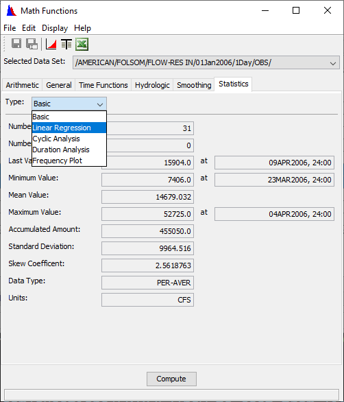
The Basic function computes the basic statistical values for a regular or irregular interval time series data set. The statistical and informational values displayed are:
Number of valid values
Number of missing values
Last valid value and date and time
Minimum value and date and time
Mean value
Maximum value and date and time
Accumulated value for the time series
Standard deviation
Skew coefficient
Data type ("INST-VAL", "INST-CUM", "PER-AVER", "PER-CUM")
Data Units ("ft", "cfs", etc.)
To compute the basic statistical parameters for a time series data set:
1. Choose the Statistics tab of the Math Functions screen and select the Basic type.
2. From the Selected Data Set list, select a time series data set.
The statistics are displayed for the time series data set once the data set is selected.
Linear Regression
The Linear Regression function computes the linear regression and other correlation coefficients between two time series data sets. Values in the primary time series data set and the second time series data set are matched by time to form data pairs for the correlation analysis. Missing values are ignored. Times for the two time series data sets must match exactly. The data sets may be either regular or irregular interval time series data.
The correlations statistics computed by the function are:
Number of Valid Values
Regression Constant
Regression Coefficient
Determination Coefficient
Standard Error of Regression
Adjusted Determination Coefficient
Adjusted Standard Error of Regression
The primary time series data set forms the values of the independent variable (x-values), while values of the second time series data set comprise the dependent variable (y-values). The linear regression coefficients express how values in the second data set can be derived from values in the primary data set:
TS2(t) = a + b * TS1(t)
where "a" is the regression constant and "b" the regression coefficient.
To compute the linear regression and correlation coefficients between two time series data sets:
1. Choose the Statistics tab of the Math Functions screen and select the Linear Regression type.
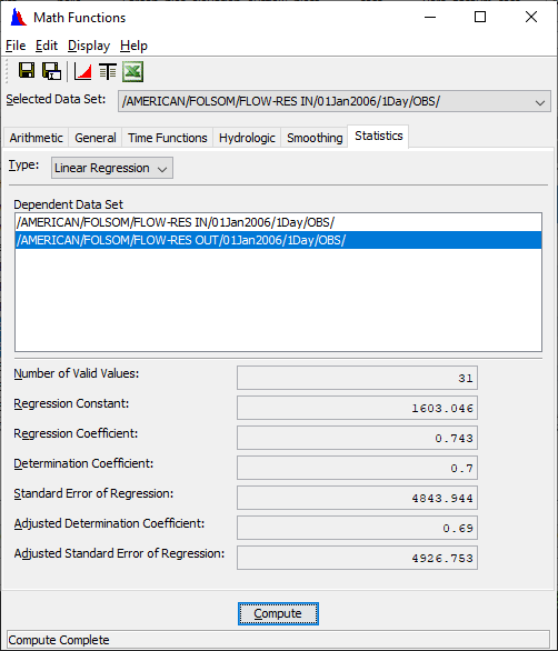
2. From the Selected Data Set list, select the primary time series data set for analysis. Time series values from this data set form the independent variable (x-values) of the correlation analysis.
3. From the Dependent Data Set list, select the second time series data set for analysis. Time series values from this data set will comprise the dependent variable (y-values) of the correlation analysis.
The correlation statistics are computed automatically once the two data sets are selected.
Cyclic Analysis
The Cyclic Analysis function derives a set of cyclic statistics from a regular interval time series data set. The time series data set must have a time interval of "1HOUR", "1DAY" or "1MONTH". The function sorts the time series values into statistical "bins" relevant to the time interval. Values for the 1HOUR interval data are sorted into twenty-four bins representing the hours of the day, 0100 to 2400. The 1DAY interval data is apportioned to 365 bins for the days of the year. The 1MONTH interval data is sorted into twelve bins for the months of the year.
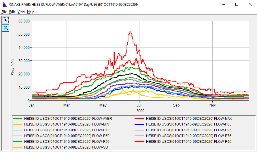
The format of the resultant data sets is as a "pseudo" time series for the year 3000. For example, the cyclic analysis of one month of hourly interval data will produce pseudo time series data sets having twenty-four hourly values for the day January 1, 3000. If the statistical parameter is the "maximum" value, then the twenty-four values represent the maximum value occurring at that hour of the day in the original time series. The cyclic analysis of daily interval data will produce pseudo time series data sets having 365 daily values for the year 3000. The cyclic analysis of monthly interval data will result in pseudo time series data sets having twelve monthly values for the year 3000.
Fourteen pseudo time series data sets are derived by the cyclic analysis function for the following statistical parameters:
Number of values processed for each time interval
Maximum value
Time of maximum value
Minimum value
Time of minimum value
Average value
Probability exceedence percentiles for 5%, 10%, 25%, 50% (median value), 75%, 90%, and 95%
Standard deviation
To compute the cyclic analysis of a time series data set:
1. Choose the Statistics tab of the Math Functions screen and select the Cyclic Analysis type.
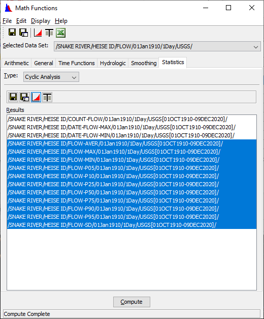
2. From the Selected Data Set list, select a time series data set for cyclic analysis.
3.Click Compute.
![]()
![]()
![]()
![]() Once the compute is performed, the resultant 14-pseudo time series data sets appear in Results list on the screen (above). One or more data sets in this list may be selected (by clicking, control-click or shift-click ) for saving to file, plotting or tabulation by using the Save button, SaveAs button, the Plot button or the Tabulate button from the toolbar located immediately above the Results list. An example showing the data plotted is shown below.
Once the compute is performed, the resultant 14-pseudo time series data sets appear in Results list on the screen (above). One or more data sets in this list may be selected (by clicking, control-click or shift-click ) for saving to file, plotting or tabulation by using the Save button, SaveAs button, the Plot button or the Tabulate button from the toolbar located immediately above the Results list. An example showing the data plotted is shown below.
Duration Analysis
The Duration Analysis function computes the duration curve for a regular interval time series data set and stores the results in a new paired data set. Flood duration curves are useful in assessing the general low flow characteristics of a stream. For example, if the lower end drops rapidly, the stream has low ground-water storage and low or no sustained flow. The overall slope of the curve is an indication of the flow variability in the stream. Refer to EM 1110-2-1415 Chapter 2 (USACE, 1993) for a description of duration analysis. Duration analysis is usually applied to daily flow or elevation or similar data. This function is not Volume Duration Frequency Analysis; see the program HEC-SSP for this capability.
HEC-DSSVue provides two techniques for computing duration curves. The first method develops the curve by ranking all the data and then extracting points along that curve. The second technique segregates values into "bins" and then plots the cumulative amount. This technique was used by the HEC-STATS program and was developed to accommodate the small amount of memory that computers used to have, or when the analysis was done by hand. Because memory limitations have been removed, the first technique is more accurate and is recommended.
The data to be analyzed must have a regular time interval of "1DAY", "1WEEK", "TRI-MONTH", "SEMI-MONTH", "1MON" or "1YEAR". Typically the time series data set for the duration analysis spans multiple years. The time series data values are first sorted by time of the year into periods of "Annual", "Quarterly", "Monthly" or "Other Defined". For an "Annual" period type, all data are assigned to a continuous single duration period. For a “Quarterly” duration period type, the data values are sorted by quarter year: 1 January to 31 March, 1 April to 30 June, 1 July to 30 September, and 01 October to 31 December. For the "Monthly" duration period type, data values are sorted by month. The "Other Defined" duration period type allows arbitrary duration periods to be defined and used.
For the standard duration analysis technique, the data values within a duration period are ranked (ordered by descending value). The ordered values form the y-values for a new paired data set. The x-values represent the percent of time exceeded computed by:
E = 100 * [ M /(n+1) ] (Weibull plotting positions), percent of the time the value is equaled or exceeded
M = the rank position of the value
n = number of values.
A curve is computed for each duration period. Thus for a duration period type "Quarterly", the paired data set has four curves with the curve labels "Jan-Mar", "Apr-Jun", "Jul-Sep" and "Oct-Dec".
The set of x-values generated by the duration analysis are dependent upon the number of values in the time series. Typically all values should be used for plotting the curve. However, this may become unwieldy when presented in a table form, so values may be a standard set of percentages, for example: 1%, 2%, 5%, 10 %, etc. If desired, the Duration Analysis function can sample the analysis results to a standard set of frequency points, or to a set of evenly distributed x-values. Using log spacing provides more clarity of the curve at its ends. User defined points can be specified by entering those points in a table after selecting the User Defined button.
To compute the duration analysis for a regular interval time series:
- Select the data set from the main HEC-DSSVue screen and then select the Math Functions button or Math Functions from the Tools menu.
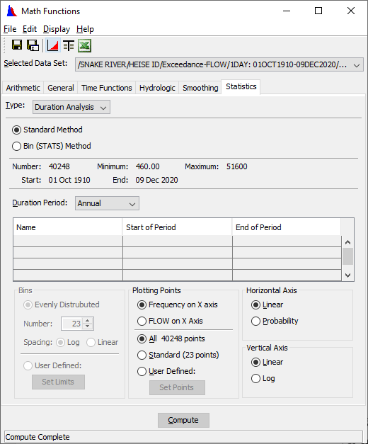
- Choose the Statistics tab of the Math Functions screen and select the Duration Analysis type.
- Select the time series data set to apply the function from the Selected Data Set pull down list
- Select either the Standard Method or Bin (STATS) Method for the analysis technique you wish to use.
- Set the duration period type using the Duration Period pull down list.
- If the duration period type "Other" is selected, the duration periods are defined in the Duration Period table. Dates entered for the "Start of Period" and "End of Period" is of the form, "05May". The duration period "Name" is assigned to the curve label in the paired data set generated by the duration analysis function.
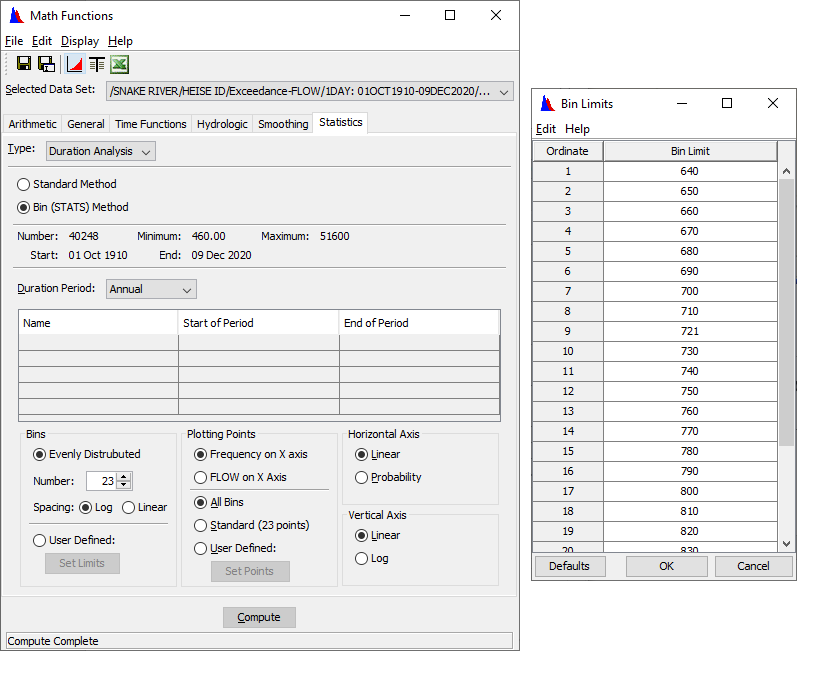
- If the Bin method is selected, choose the number of bins to use, and if those bins should be spaced log arithmetically or linearly between the minimum and maximum values. Or select User Defined bins and enter values into the table by pressing the Set Limits button, as shown below. User defined limits will provide greater flexibility to select the parameter values desired.
- The values provided in the table are either those computed using the number of bins and spacing method selected before, or those saved from the previous run. To reset the values to the default ones, press the Defaults button. This will use the number of values selected to compute the default values. An example of the Bin Limits table is shown below.
- Select whether you want the Frequency to be on the X axis or the Parameter on the X axis. Typically Frequency is given on the X axis. If you display the results in tabular form, you may want to select the parameter for the X axis.
- The number of duration points retained for plotting and tabulation is controlled by the Plotting Points options. Select the All Bins radio button to retain all the ranked computed duration points. Select the Standard radio button to interpolate the results to the traditional set of 23 log points. You may choose your own number of points by selecting the User Defined radio button and entering the desired number of interpolation points in the box to the right. Select either Log or Linear spacing on where to sample those points.
- The Horizontal and Vertical Axis options control the scales for plotting the duration analysis curves. The Linear scale radio button selects a linear plot scale for the both the x and y axes. The Probability scale radio button selects a probability scale for the x-axis and a log scale for the y-axis.
- Click Compute. Note: any change to the plot configuration requires a re-compute of the data.
- Select the plot button to view the computed duration curve(s). An example of resulting plots are shown below.
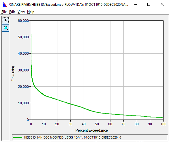
Linear Vertical and Horizontal Axis
Linear Vertical and Log Horizontal Axis
- You can also select to view the data as tabular or display in Microsoft Excel. The table in Figure 7.48 below was computed by using the bin method for monthly periods and tabulating with Elevation on the X axis.
Figure 7.48 Monthly Exceedences for Elevations
Frequency Plot
The Frequency Plot function computes and displays a frequency plot for a peak annual data from a time series data set. This computation is intended for period of record (years) of primarily stream flow data. The data can be in intervals less than year, as annual peaks are automatically calculated from the data set. The plot is generated by computing annual peaks from the data set and then ranking the data and plotting. An optional curve may be drawn for your data set using the Log-Pearson type III transformation equation as described in Bulletin 17B.
Calculation Outline:
* get annual peaks (calendar year Jan1-Dec31)
* zeros removed
* Converts all values to Log10 space
* computes mean, variance, std, and skew
* computes k value using equation from 17-B https://water.usgs.gov/osw/bulletin17b/dl_flow.pdf
* computes flows for standard probability ordinates using Log Pearson III
* outliers dropped using Grubbs-Beck test from Bulletin 17B
For a detailed frequency analysis with additional parameter control, the user is referred to the program HEC-SSP. The HEC-DSSVue computation provides a quick evaluation of data.
To compute a Frequency Plot for a time series set:
1.Select the data set from the main HEC-DSSVue screen and then select the Math Functions button or Math Functions from the Tools menu.
2.Choose the Statistics tab of the Math Functions screen and select the Frequency Plot type, as shown below.

3.Select the time series data set to apply the function from the Selected Data Set pull down list.
4.Select the checkbox Show computed curve with observed points if you wish to.
5.Press Compute.
If needed a message about outliers will appear:
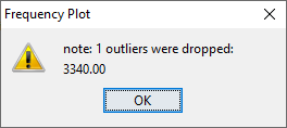
6.A plot will be displayed showing the frequency plot and computed curve (if selected), which is shown below.
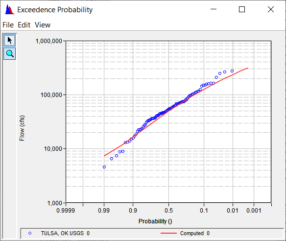
Frequency Plot and Computed Curve for Daily Flow Data