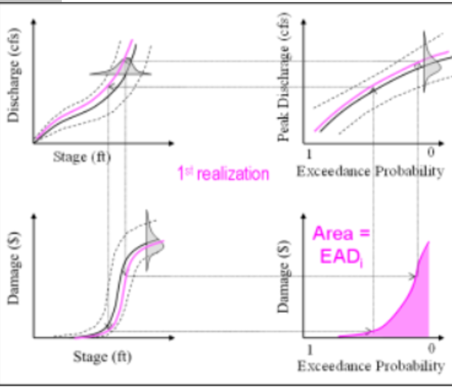
Expected Annual Damage with Uncertainty
Uncertainty in Risk Assessments
Economic risk assessments, require explicit consideration of the uncertainties associated with key hydrologic, hydraulic, and geotechnical variables and the character of floodplain occupancy (ER 1105-2-101). The risk assessment and study effort should concentrate on the uncertainties of those variables which have a significant impact on study conclusions and recommendations (ER 1105-2-101). This focus can be accomplished by determining the best estimate of each of the functions used for risk computation, and then describing the uncertainty over the range of the function.
Each of the summary relations (hydrology, hydraulics and economics, etc.) that we use to measure risk comes with uncertainty. Take for instance the hydrologic summary (discharge frequency) curve, there is imperfect knowledge about which probability distribution model will fit the natural variations of flow data and there is also uncertainty regarding the appropriate values of the distribution parameters for that model. In other words, quantitative models used to represent reality are limited by the inability of the theory to model the complex nature of the processes we attempt to model. Because of this, our estimates of interest, whether economic or engineering, will too be uncertain. One way to reduce the impact of uncertainty is to define the uncertainty around each input summary curve and incorporate its accompanying uncertainty directly into the analysis. The result is a risk and uncertainty assessment that allows calculation of metrics such as EAD with uncertainty, AEP with uncertainty, and assurance.
Uncertainty can be included explicitly in the analysis by assuming a best-fit probability density distribution to describe the range of likely functions. Practically, computations for a risk and uncertainty assessment may be accomplished with Monte Carlo simulation. A useful way to describe Monte Carlo analysis is that it replaces a probability distribution by a very large, random sample of values from that distribution, and evaluates each sample member to form a new sample of the analysis result . USACE typically employs either of two Monte Carlo approaches in the agency’s risk assessment software: “curve sampling” or “event sampling.” This section describes the “curve sampling” approach to estimating expected annual damage with uncertainty.
EAD with Uncertainty
The curve sampling approach uses random sampling to perturb each summary function (or, curve) in the risk computation within its uncertainty, producing a “realization” of each function. Each entire function (discharge-frequency, discharge-stage and stage-damage, etc.) is replaced by the randomly sampled function to produce a large sample of output curves. Recall from the curve combination discussion above, in order to accomplish risk computation, we matched peak flow of a certain frequency and related that flow to a stage then related that stage to a point on the stage damage curve for all frequencies to develop a probability distribution for damages (a damage frequency curve). The Monte Carlo curve sampling process does the same thing but rather than a point-to-point relation, the process samples an entire curve within its range of uncertainty.
HEC-FDA uses this Monte Carlo simulation to generate a new iteration of a curve by randomly selecting parameters within uncertainty bands surrounding the curve. When we randomly select the parameters representing, for example, a flow frequency curve, we are allowing the curve to vary randomly modeling the random nature of hydrologic events. Each time we do that we have a new curve to draw from. To carry out the process, we randomize parameters for every summary relationship thereby drawing new curves from which to estimate EAD. We continue the process for many iterations to develop a sample of EAD which when graphed can be described using measures of central tendency and spread (i.e., mean and percentile). The sample of EAD represents all of the uncertainty inherent in the inputs used in the estimate.
The figure below illustrates the process for one realization of curve sampling, which produces one estimate of EAD. The bounds of uncertainty and distribution are represented by the bell-shaped curves and the dotted lines. With repeated random sampling (Monte Carlo analysis), the distributions of uncertainty are reproduced to explicitly capture the uncertainty in the risk computation and risk metrics. Thousands of realizations are needed to fully reproduce the uncertainty around each function and thus around EAD (and system performance metrics, e.g., AEP).

With repeated random sampling (a Monte Carlo analysis), the distributions of uncertainty are reproduced to explicitly capture the uncertainty in the risk computation and risk metrics. Thousands of realizations are needed to fully reproduce the uncertainty around each function and thus around EAD and system performance metrics (e.g. AEP). The figure below shows a sample of EAD estimates resulting from the Monte Carlo analysis, describing the impact of the knowledge uncertainties on EAD.
