This section details the computational procedures used by HEC-FIA to convert hydraulic data into summary information at point locations across a floodplain. The procedures used depend upon the type(s) of inundation data input to the model. The computational procedure for each of the four types of inundation data are described in the following subsections.

Cross Sections/Storage Areas

The following procedures discuss how cross sectional inundation data is applied to point locations. The internal procedure used by HEC-FIA to calculate flood depths at point locations is described in this section. The procedure used to compute other hydraulic characteristics is generally the same.
To facilitate a description of the general process by which cross sectional inundation data is applied to a point location, a generic hydrograph with example parameters is displayed in figure below (Cross Sections Only). The lowest horizontal dashed line represents the ground surface elevation (GSE); the middle horizontal dashed line represents the elevation computed by adding the non-evacuation threshold to the GSE; and, the highest horizontal dashed line represents the maximum water surface elevation (WSE). For structures, the non-evacuation elevation is equal to the foundation height (FH). The difference between the maximum WSE line and the GSE line is the maximum inundation depth at a structure.

Cross Sections Only - Event Computations using Cross Section Inundation Data

In the figure above, the T1 vertical dashed line represents the first time at which the WSE exceeds the GSE at a structure. The T2 middle horizontal dashed line represents the time at which the WSE exceeds the non-evacuation elevation. The right-most vertical dashed line, T3, represents the final time at which the WSE exceeds the GSE. The difference between T3 and T1 represents the duration of flooding for agricultural purposes, while the difference between T3 and T2 represents the duration of flooding for ECAM calculations.
An example of how to assign cross section data to an individual structure will now be explained. The figure below ("Generic Cross Section Layout") displays a simple cross section layout, with the black lines representing cross sections and the yellow line representing the stream centerline. From a storage area shapefile (not required), the geographic extents for the storage area-linked hydrographs could be applied.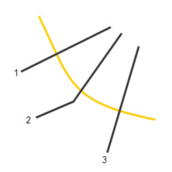

Generic Cross Section Layout

During a compute, time-series information (e.g., stage, arrival time) is read from a DSS file at each cross section and storage area. To support this compute process, HEC-FIA needs to link the geographic location, naming convention, and a DSS file path to the shapefile attributes of each cross section and storage area. For detail on the linking of DSS time-series to cross sections and storage areas, see Watershed in the HEC-FIA User's Manual. During the compute, HEC-FIA will sort the cross sections based on the River Name and River Station attributes to ensure that structures between two cross sections are assigned to the correct hydrograph data (Figure Below). When storage areas are used, similar information is required to link the storage area shapefile to the hydrographs, using the same DSS file that linked the cross sections to the storage area hydrographs.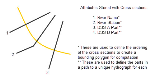

Cross Section Shapefile Attributes and DSS File Mapping
Hydraulic characteristics in the regions between cross sections are linearly interpolated based on the hydraulic characteristics of the bounding cross sections. To interpolate the results from the cross sections to a structure located between the cross sections, the cross sections are first sorted by River Name, then by River Station. The ends of each cross section are connected with a straight line to form polygons that group structures. Within the corresponding upstream and downstream cross sections, any structures that fall outside a polygon will not be considered in the HEC-FIA simulation. For example, the figure below displays two cross section bounding polygons, with the black lines representing cross sections, the yellow line representing the stream centerline, and the dotted blue lines representing the edges of the cross section polygons.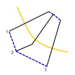

Cross Section Bounding Polygon Creation
The bounding polygon scheme can result in issues, particularly near river confluences (as seen in the figure below). Polygons may not be created for some areas, resulting in missing data (red shading). In other areas, polygons may overlap (orange shading in below figure), in which case the depth will be considered for only one polygon. The modeler should check for these issues and correct as needed.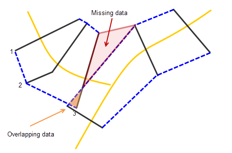

Common Bounding Polygon Creation Issues at Confluence
If a structure is within more than one bounding cross section polygon (e.g., from overlapping data), HEC-FIA defaults to using the first river in the list of alphabetically sorted rivers. If data should be assigned to a river other than the one selected by default, then the user will need to manually assign the correct river to structures within overlapping polygons in the shapefile.
Polygon creation issues can also arise near sharp river bends (as seen in the figure below). If a bend occurs between two cross sections and the cross sections do not extend far enough into the overbank, the bounding polygon may not cover the intended area. To remedy this situation, additional cross sections should be added to define the bounding polygon extents more appropriately.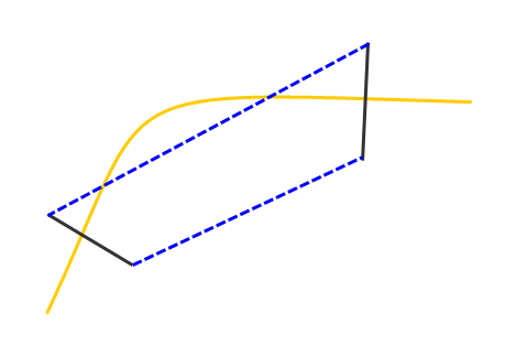

Common Bounding Polygon Creation Issues at River Bend
The distance from each structure to its bounding cross sections is calculated by HEC-FIA, using a shortest distance algorithm, which is illustrated in the figure below. The distance to the upstream cross section is added to the distance to the downstream cross section (x1 plus x2), and this value is used as the interpolation distance. The hydraulic properties for the individual structure is then interpolated between the properties of the upstream and downstream cross sections.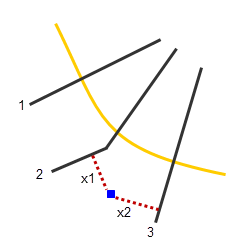

Shortest Distance Determination
As an example, assume that HEC-FIA calculates the River Station (RS) of a structure to be located at RS 1175. The structure is bounded by a cross section located at RS 1200 and a cross section located at RS 1100. The cross section at RS 1200 has a maximum WSE of ten feet, while the cross section located at RS 1100 has a maximum WSE of six feet. Therefore, a linear interpolation of the WSE to the structure located at RS 1175, means that the structure will be modeled as experiencing a maximum WSE of nine feet.
Because the depth of flooding at a structure is computed by subtracting the structure elevation from the WSE when using cross section data, it is possible for HEC-FIA to compute structures with basements as being flooded. For example, if the WSE at a structure is 100 feet and the structure elevation is 102 feet, the calculated depth at the structure is negative two feet. If this structure has a basement that extends five feet below the GSE, the basement will be modeled as being inundated by three feet of water, which would result in damage being calculated for the structure even if the first floor elevation was above the calculated WSE.
Assigning hydrographs to structures is significantly simpler when the structures are located within a storage area. The DSS hydrograph associated with the storage area is imported into HEC-FIA and assigned to each structure located within the storage area polygon.

Grids

The algorithm used to apply flood depth data to structures is described in this section. However, the algorithm is general enough to describe the process through which every type of hydraulic information is applied to structures. To describe the general approach in which the inundation data from grids is applied to structures, a generic grid schematic with structures is provided in the figure below. For example, the figure displays an inundation depth grid, with the depths of each grid cell represented by the blue numbers and two buildings represented by the red polygons. Note that building locations are reduced to points in HEC-FIA; the buildings were drawn as polygons in the figure solely for illustrative purposes.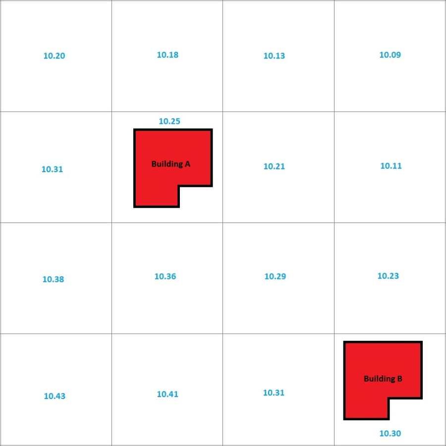

Event Computations using Grid Inundation Data

A hydraulic characteristic is assigned to buildings based on the value of the grid cell in which the point representing the building is contained. Each structure is represented as a discrete point, which is typically the centroid of a parcel shapefile; therefore, each structure exists in a single grid cell even if the parcel covers many grid cells. Interpolation of hydraulic characteristics is not necessary due to this assignment methodology. Using the example in the figure above, an inundation depth of 10.25 feet would be assigned to Building A and an inundation depth of 10.30 feet would be assigned to Building B. The same procedures are followed for all of the types of gridded data that can be accessed by HEC-FIA.
Because the depth of flooding at a structure is computed in HEC-FIA for gridded data directly from the provided grid (which represents depth above the GSE), it is not possible for HEC-FIA to compute structures as only having basements inundated. When using gridded data, the basement will be either completely dry or completely wet, depending upon whether a positive depth is noted in the inundation grid cell corresponding to the building location.
The same hydraulic information is assigned to all structures within any given grid, regardless of the structure's position within that grid. Therefore, the accuracy of the assigned hydraulic data is a function of the degree to which the hydraulic data is constant across the portion of each grid containing structures.

Grids and Cross Sections/Storage Areas

The grids and cross sections/storage areas computational procedures depend upon the amount of data that is provided as a grid. Structures will be assigned hydraulic characteristics first based on the gridded data, using the computational procedures outlined in Grids. After all gridded data inputs have been assigned, HEC-FIA will use the computational procedures outlined in Cross Sections and Storage Areas to determine the depth and arrival time for each structure, as necessary.
To describe the general approach in which the inundation data from cross sections is applied to structures, a generic hydrograph is provided. The figure below displays the generic hydrograph along with key parameters. The lowest horizontal dashed line represents the GSE, the middle horizontal dashed line represents the elevation computed by adding the non-evacuation threshold to the GSE, and the highest horizontal dashed line represents the maximum WSE. If gridded data is supplied, the value at each structure will be taken from the grid. If not, the inundation depth will be determined from the cross section data as the difference between the maximum WSE line and the GSE line.
In the figure below, the left-most vertical dashed line, T1, represents the first time at which the WSE exceeds the GSE. The middle horizontal dashed line, T2, represents the time at which the WSE exceeds the non-evacuation elevation. The right-most vertical dashed line, T3, represents the final time at which the WSE exceeds the GSE. The difference between the T3 and T1 lines represents the duration of flooding for agricultural purposes, while the difference between the T3 and T2 lines represents the duration of flooding for ECAM calculations.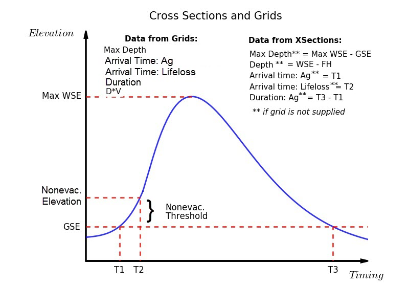

Event Computations using Grid and Cross Section Inundation Data

Common Computation Points (CCPs)

The general methodology used by HEC-FIA for applying inundation data from the common computation points to the structures is displayed in the figure below. In general, inundation data for each structure is determined using common computation points in a similar manner to using cross sections.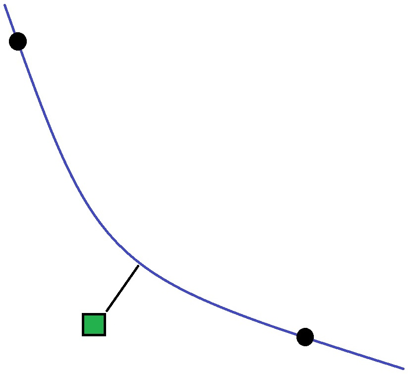

Common Computation Points Methodology Example
The first step in the process is to calculate the stationing of the common computation points (black points in the above figure). Each common computation point is located directly on the stream alignment centerline (blue line in the above figure), which allows for a straightforward river station calculation. Next, the stationing of each structure (green box in above figure) is determined by interpolating between the upstream and downstream common computation points. The interpolation uses the shortest distance algorithm, as described previously, whereby the stationing is determined from where a straight line drawn from the structure and perpendicular to the stream alignment crosses the stream alignment (black line in above figure). Finally, using the stationing of the upstream and downstream common computation points and the stationing of each structure, the inundation data from the hydrographs linked to each common computation point can be interpolated for each structure, based on that structure's stream stationing.
A difference between the common computation point and cross section/storage area interpolation methodology is that no boundary is established for how far away from the stream the common computation point is valid. While the cross section data is limited to the extent of the cross section shapefile and the storage area data is limited to the extent of the storage area shapefile, the point nature of the common computation points does not allow a known extent to be established. While this approach eliminates the possibility of some of the potential errors discussed in the cross section methodology section, the approach can cause unusual results.

For the example, in the figure below, the structure (green box) is located on the landward side of a high ridge (represented by the red line) separating a river (blue line) from the structure. The structure would take on the stage attribute of the river, even though water cannot actually reach the structure due to the ridge being higher than the river stage. This issue is less likely to occur when using cross sections, as the cross sections and resulting bounding polygon would likely end at the high ridge. The possibility of this issue occurring when using cross sections can be limited by using an appropriate hydraulic model setup. If the high ground issue does cause problems in the HEC-FIA modeling, HEC-FIA includes a "High Ground Tool" for editing watersheds. This HEC-FIA tool is available in the HEC- FIA map window toolbar when the Watershed Configuration is displayed in an HEC-FIA map window. The High Ground Tool allows the user to define a polygon that is behind high ground, and provides the stationing of the overtopping location and the overtopping elevation. After the threshold is met at the overtopping station, all structures in the polygon are flooded based on each structure's depth from either the gridded or the cross section data.
Because the depth of flooding at a structure is computed by subtracting the structure elevation from the WSE when using common computation point data, it is possible for HEC-FIA to compute structures with basements as being flooded, even if the stage fails to reach the GSE at the structure. HEC-FIA will compute damage for each structure to the lowest ordinate on the depth-damage curve that is associated with the occupancy type for each structure.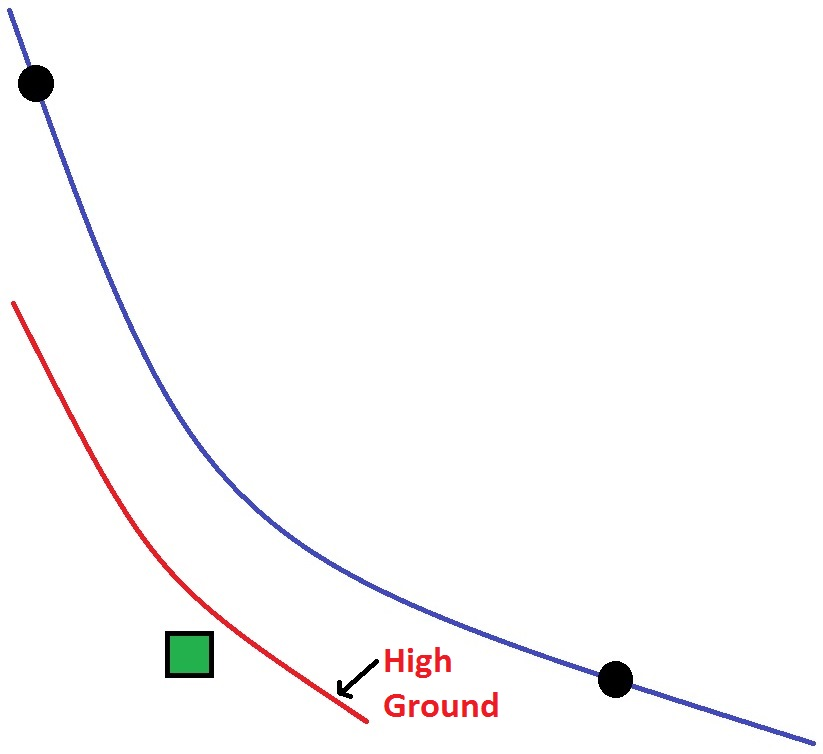

Common Computation Points Potential Error