Two computational inputs are required for HEC-FIA to conduct a Monte Carlo simulation:
1) continuous distributions, and 2) Monte Carlo application controls. Relevant information about each input data type is contained in this section.

Continuous Distributions

All distributions used in HEC-FIA are continuous distributions. The continuous distributions are used to convert a randomly drawn number into a value that is transformed through the distribution, which is the basis of the HEC-FIA Monte Carlo algorithm. In the Monte Carlo algorithm, the inverse of the cumulative distribution function is utilized to find a randomly distributed value that can be used as an input to the deterministic mathematical function describing the desired relationship. Four different forms of continuous distributions can be selected in HEC-FIA: 1) uniform; 2) triangular; 3) normal; and, 4) log normal.
Any of the four continuous distributions can be defined for a number of parameters and inputs to HEC-FIA. A list of the parameters and inputs for which a continuous distribution can be specified in HEC-FIA is shown listed:

Structure, Content, Other, and Vehicle Depth-Damage Functions
Foundation Height
Structure Value as percent of Mean
Content to Structure Value Ratio (percent)
Other to Structure Value Ratio (percent)
Vehicle to Structure Value Ratio (percent)
Warning Issuance Delay time
Time-Percent Mobilization Functions

The four different forms of continuous distributions are described in the following sections.

Uniform Distribution

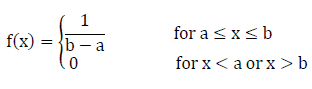
The uniform distribution is the most basic of the four distributions. The two required input parameters for the uniform distribution are the maximum and minimum possible values for the parameter of interest. The maximum and minimum values may be any real number. The Probability Density Function (PDF) of a uniform distribution is shown in the figure below. The PDF is described mathematically in the equation below, where a is the minimum and b is the maximum value of x.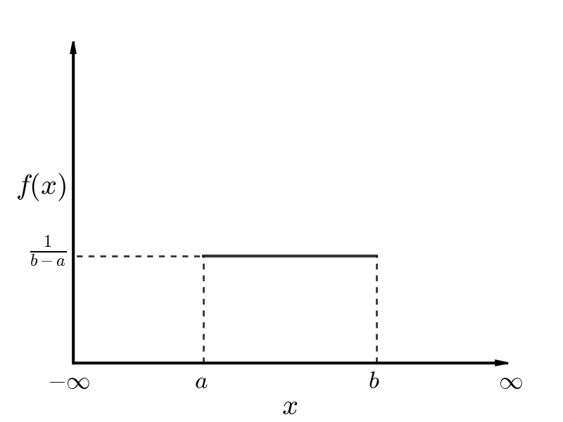

Probability Density Function (PDF) of a Uniform Distribution

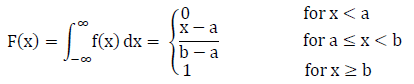
The Cumulative Distribution Function (CDF) of a uniform distribution is shown in the figure below. The CDF is described mathematically in the equation below: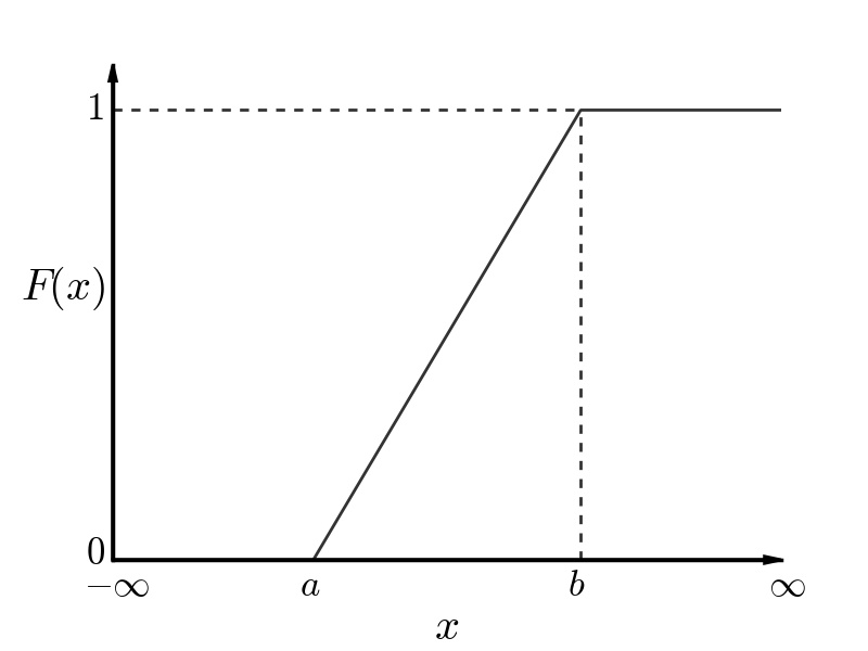

Cumulative Distribution Function (CDF) of a Uniform Distribution

Solving for x in the solution space of (0,1], the inverse CDF for the continuous uniform distribution is shown in the equation below:

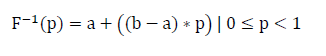
Triangular Distribution

A triangular distribution requires that the minimum, maximum, and mode values of the parameter of interest be entered into HEC-FIA. Note that the mode value may or may not be the mean of the distribution, and must fall between the minimum and maximum values. The PDF of a triangular distribution is shown in the figure below. The PDF is described mathematically in the equation below, with the assumption that a ≤ c ≤ b.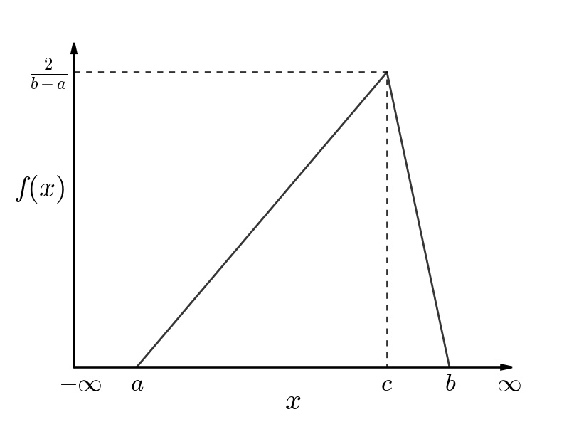

Probability Density Function (PDF) of a Triangular Distribution

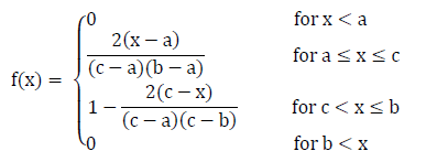
The Cumulative Distribution Function (CDF) of a triangular distribution is shown in the figure below (assuming that a ≤ c ≤ b.), and is described mathematically in the equation below.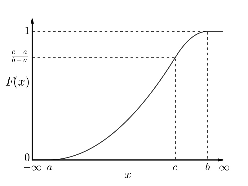

Cumulative Distribution Function (CDF) of a Triangular Distribution

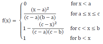
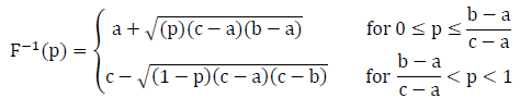
The inverse cumulative distribution for a triangular distribution, given a ≤ c ≤ b, is as follows:

Normal Distribution

The normal distribution is one of the most commonly used distributions in evaluating uncertainty. HEC-FIA requires that the mean (µ) and the standard deviation (σ) of the distribution be specified. In a normal distribution, the value range is always negative infinity to positive infinity, so it is important to consider the repercussions of choosing this distribution.
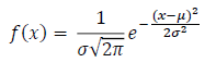
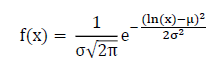
The PDF of a normal distribution is displayed in the figure below, and is described mathematically in terms of µ and σ in the equation below.

Probability Density Function (PDF) of a Normal Distribution

The CDF of a normal distribution is displayed in the figure below and described mathematically in the equation below.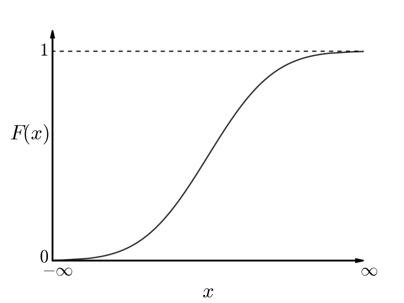

Cumulative Distribution Function (CDF) of a Normal Distribution

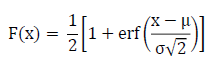
The error function, denoted as erf(x) in the above equation, is an integral that cannot be expressed in elementary functions and can only be approximated. To determine the inverse of this function requires an approximation as well. To evaluate the inverse CDF, a Taylor series polynomial is used to approximate the normal distribution.
The t value is only evaluated from zero to 0.5, so if p is greater than 0.5, the value 1-p is evaluated in t. This assumption is appropriate given that the normal distribution is symmetrical. The inverse CDF for a normal distribution is shown in the equation below.

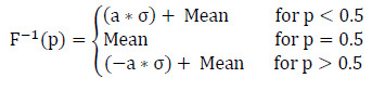
Where a is defined in the following equation as:

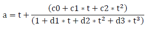
where:
c0 = 2.515517
c1 = 0.802853
c2 = 0.010328
d1 = 1.432788
d2 = 0.189269
d3 = 0.001308

$\begin{array}{l}\displaystyle t = \sqrt(ln(1/p^2))\end{array}$

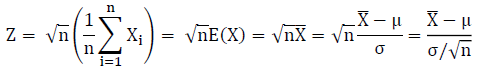
The standard normal distribution, where mean (µ) = 0 and standard deviation (σ) = 1, is generally expressed as Z as shown in the equation below.

Log Normal Distribution

A variable x is log-normally distributed if ln(x) is normally distributed. Log normal distribution is often used to assist in parameterizing random variables that are always greater than zero.
HEC-FIA requires that the mean (µ) and the log₁₀ of the standard deviation (σ) be specified for this distribution. The PDF of the log normal distribution is described mathematically in terms of µ and σ and is described in the equation below.

The CDF of the log normal distribution is described mathematically in the following equation:

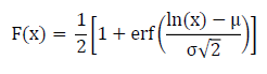
The inverse CDF is a simple transformation of the normal distribution CDF and is shown in the following equation:

Monte Carlo Controls

Three input variables are required for the Monte Carlo simulation in HEC-FIA. The first input variable, Initial Seed, is used in the random number generator to create a uniformly distributed pseudo random number sequence. The pseudo random number sequence will be duplicated if the same Initial Seed value is used, which ensures that results in HEC-FIA are repeatable. The default Initial Seed value is 0.

The second input variable, Convergence Tolerance, is used to specify when the Monte Carlo has reached the established criteria for convergence. A smaller Convergence Tolerance will yield more iterations and potentially provide a more reliable output distribution. The default Convergence Tolerance value is 0.05.

The third and final input variable required by HEC-FIA is the Convergence Confidence Interval. This variable is used in conjunction with the Convergence Confidence Tolerance to define the alpha (α) value in the tail of the output distribution for which to track convergence.

Evaluating Convergence

It is important for the HEC-FIA user to evaluate the number of runs needed to get a reasonable representation of the result space. Convergence testing is used to determine when sufficient runs have been computed. The approach used is to evaluate the change in the mean value of the sample space from one run to the next.
A simple way to test for convergence is to compare the mean from the previous sample set to the new sample mean with the addition of each additional simulated result. The test would evaluate when the change in value is less than some critical threshold (shown in the equation below).

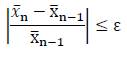
The above equation is a test that simply evaluates the slope of the running average and compares the slope to some arbitrarily small positive quantity, ε. The theory is that if the slope of the running average is approaching zero, the average is not changing any longer, and the sample size is large enough that the additional sample is no longer capable of influencing the mean.
While this test describes convergence testing at its simplest, convergence is not a very good test since it is possible for the next sampled value to be close enough to the mean that its value is not enough to change the running average, thus exiting the Monte Carlo early. To overcome this possibility, tests that are more stringent are used in HEC-FIA.

Sample Size Selection

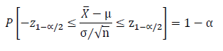
Sample size for each parameter is selected based on an evaluation of how far a value can be from the mean to be within a specified tolerance level, with a specified amount of confidence. A confidence interval can be expressed with the equation below and is graphically described in the figure below.

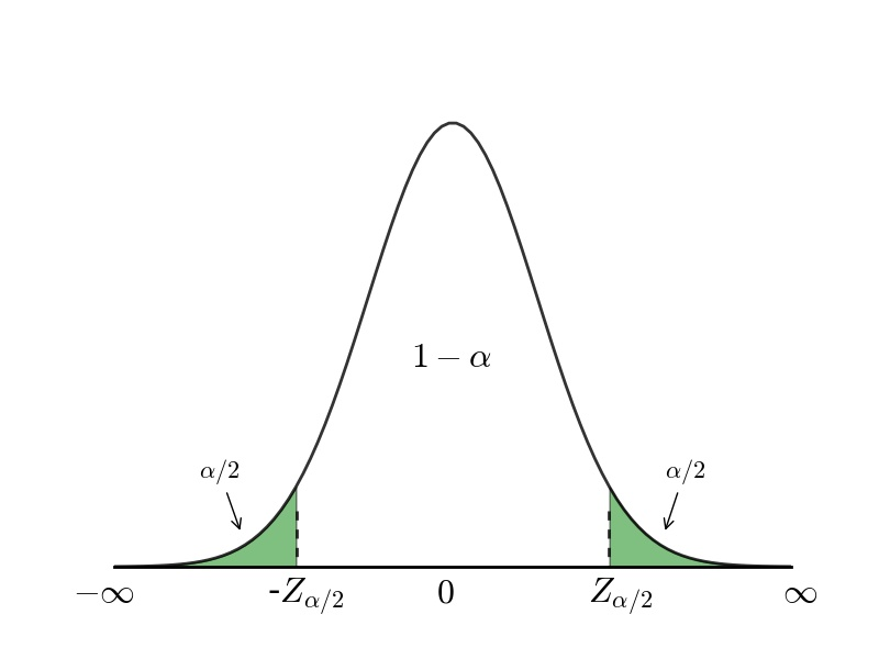
Confidence Intervals for a Standard Normal Distribution

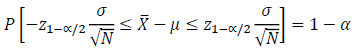
The inequality (above equation) is then simplified by replacing Z using the Central Limit theorem (figure below).

Which yields the following:

The following equation is then produced after rearranging within the inequality by multiplying all terms by σ/√N:

The population standard deviation in the above equation, σ, is substituted with S, which is the estimate of the standard deviation from the sample of size N, to produce Equation the following equation.

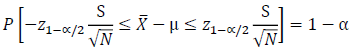
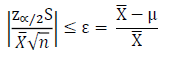
Thus, the resulting expression (above equation) yields a 1-α probability that the sample mean is less than the distance of the estimate is from the true mean (equation below).

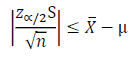
The minimum distance threshold from the true mean can be specified by setting an acceptable value for the error. For this example, the error is _X-μ (above equation). However, the error could alternatively be represented as a percentage of the mean estimate, which would be as follows in the equation below:

Expressing the error as a percentage, allows the calculation to be evaluated regardless of the magnitude of the random variable (equation below).

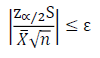
Since neither the sample mean, X, nor the sample standard deviation, S, known a priori, this equation must be evaluated at the completion of every iteration. Once the equation becomes true, sufficient samples have been made to conclude that the sample mean is within ε distance from the true mean with 1-α confidence.

Random Numbers and Seeds

To evaluate any of the inverse CDF functions described above in a Monte Carlo simulation, it is imperative that the input probabilities for each of the sampled random variables be random and uniformly distributed. The assumption that the probability of any given random variable is equal to 1/n (where n is the number of random variates drawn) is predicated on the fact that any probability of any of the random variates occurring is equally likely to occur. Any resulting parameter is distributed as described by the functional relationship and the distributions of any input parameters.
To accomplish this goal, a random number generator is utilized. Pseudo random numbers are created in many ways. The approach implemented by the Java platform and utilized by most HEC software is described here. This random number generator creates a uniformly distributed pseudo random number sequence that can be duplicated if the same seed is used.
The method deployed by Java is a linearly congruential method, as described by D. H. Lehmer and described by Donald E. Knuth in The Art of Computer Programming, Volume 3: Seminumerical Algorithms, Section 3.2.1 (Appendix A). The random number generator is described by the following relation in the equation below:

where X_n is the sequence of pseudo random variables, a and b are the multiplier and increment, and m is the modulus, which is the value describing the divisor in modular arithmetic. In the Java library the values of a, b and m are fixed (as defined below); however, the value X₀ can be set by the user and is generally referred to as the "seed".

a = 25214903917
b = 11
m = 2⁴⁸

In the random number generator relation described in the equation above the general meaning of congruent modular numbers is that the values on each side of the "≡" have the same remainder when divided by the modulus (m). In computer calculations, the method to determine the remainder is more difficult than the division to do a byte shift on a binary representation of a number; therefore, the modulus (m) is chosen to be an exponent of two so that the remainder can be calculated by removing the exponent number of bytes from the right of the array. The results of this byte shift method is equivalent to dividing by the modulus value. However, the equation above will always equate to an integer value. To convert the integer value to a number between (0,1), two numbers are drawn and then a modulus of 2²⁷ is drawn; the numbers are then combined as one number (concatenation of the bytes for lack of a better description) and divided by 2⁵³. Therefore, the value of X_n+1 is entirely predicated on X₀ (or "seed") and the current value of n.
The actual process that the number generator uses to create the next integer relies on the truncation of bits from the right (in Java's case the last 48 bits in the sequence) which is equivalent to modular division.