The Monte Carlo simulation procedures are described in the steps below.

1. Create a uniformly distributed pseudo random number sequence based on the initial seed value entered by the user as a Monte Carlo control.
   
   
2. Calculate economic damage and life loss results for each random number in the sequence, based on the continuous distribution type selected and the related input parameters for that distribution.
   
   
3. Test for convergence within the user-specified confidence interval.
   
   
4. If convergence has not occurred within the user-specified confidence interval, repeat Steps 1 through 3 until convergence is obtained.

In the above procedures, Step 2 requires sampling of the continuous distribution and in HEC-FIA, there are four sampling techniques available. The four sampling techniques are: single parameter, two parameter, tabular relationship, and standard deviation as a percentage of the mean. Moreover, the sampling technique utilized by HEC-FIA depends on the input parameter and how that parameter relates to the Monte Carlo computational procedure overall. For instance, depth damage relationships are sampled using tabular relationship sampling, while foundation heights are sampled using single parameter sampling. Furthermore, each technique samples a value from the CDF by utilizing the random numbers provided in Step 1, and then selects a value based on the provided random number. The following sections discuss the procedures for the four possible sampling techniques used by HEC-FIA in Step 2.

Single Parameter Sampling Technique

If one input variable is described by a continuous distribution, the CDF samples that single parameter using the single parameter sampling technique. As an example, if parameter x is triangularly distributed with a minimum value of 0.0, a mode value of 0.5, and a maximum value of 1.0, the following inverse CDF will be produced as shown in the following equation:

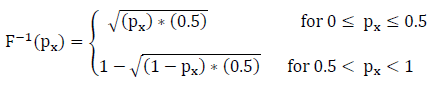
Assuming an input set of p_x values of {0.1, 0.4, 0.7, 0.8}, the CDF sampling would result in a solution set of {0.223607, 0.447214, 0.612702, 0.683772}, respectively.

The solution set is evaluated for a constant value with respect to the parameter d (equation below):

For example, assuming d = 5 and using the above equation, the following values would be obtained:

Two Parameter Sampling Technique

If two input variables are described by a continuous distribution, the two parameter sampling technique is used. As an example, if parameter d (as described in the above section) is assumed to be triangularly distributed, rather than a constant value, and has a minimum value of 4.0, a mode value of 5.0, and a maximum value of 7.0, the following inverse CDF will be produced for parameter d as shown in the equation below:

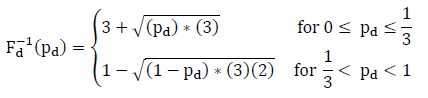
Next, the solution set obtained is evaluated for parameters d and x using the equation below:

If p_d = {0.45, 0.24, 0.31, 0.85} and p_x = {0.1, 0.4, 0.7, 0.8}, the result would be the following solution sets:

 

Using the preceding solution sets and equations, the following values would be obtained:

As more parameters are defined with uncertainty, the computational complexity of these functions becomes exceedingly more difficult.

Tabular Relationship Sampling Technique

To compute uncertainty associated with a tabular relationship, HEC-FIA employs sampling techniques to obtain tabular relationships that maintain a certain required criteria. An example of a required criteria is that the tabular relationship is monotonically increasing, or that the maximum value cannot be greater than 100.
Therefore, to compute uncertainty, the curve characterizing the tabular relationship is represented as a collection of distributions, with one distribution for each ordinate. A single probability is sampled for all of the distributions and a curve is created for each ordinate. For example, a minimum, maximum, and most likely (Y) value are used to describe the triangular distribution for each X ordinate. The example (Y) values and X ordinates are listed in the table below, while the figure below plots the curves for each of these example values.

Example Values Used to Describe Triangular Distribution

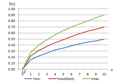
Curves Used to Describe Triangular Distribution Example

For this type of tabular relationship sampling, the probability value is provided one time per Monte Carlo iteration, yielding an entirely new curve. Within each Monte Carlo iteration, the probability value is held constant. As a result, all X ordinates used within the iteration are drawn from the same probability for each distribution within the tabular function; an example result is shown as a purple line in the figure below.

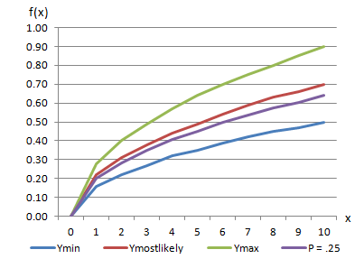
Curves Used to Describe Triangular Distribution Example for a Probability Value of 0.25

In addition to the resulting curve (above figure), The figure below also provides an example result (also drawn as the purple line). For these two examples, the above figure displays the curves for the probability value 0.25, while the below figure shows the curves for the probability value 0.05.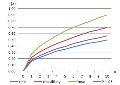 


Curves Used to Describe Triangular Distribution Example for a Probability Value of 0.05

Standard Deviation as a Percentage of the Mean Sampling Technique

The final typical sampling technique employed in a Monte Carlo simulation is to evaluate a group of values' relative deviations from their respective means. This evaluation is beneficial when a consistent measure of error in the parameter exists. Examples may be structure values, rock sizes, foundation heights, and flow values measured by the same flow gage, among others. This type of sampling allows a consistent percentage error to be applied across all items of the same type.

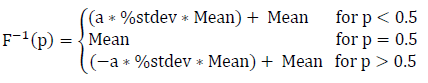
The evaluation is similar to a standard single parameter sample; however, the magnitude of the mean is inserted into the equation and instead of a typical standard deviation, the standard deviation is expressed as a percentage of the mean. For example, if assuming a normal distribution, the mean value is described for each random variable, and the standard deviation (stdev) is expressed as a percentage (%stdev) of the mean. Therefore,
stdev = %stdev * Mean and the equation is shown as: