Fragmentation in habitat maps produced by the EFM process is generated by land surface topography that affect the connectedness of aquatic habitats through human or natural features, splicing of multiple layers into a habitat mosaic, and application of habitat suitability criteria that split otherwise connected areas into smaller pieces surrounded by areas with zero suitability.
In GIS, raster datasets are grids of continuous cells organized in rows and columns. Areas with raster values can be separated by areas of no data. Connected raster cells that provide habitat are herein called “chunks” (Figure 35).
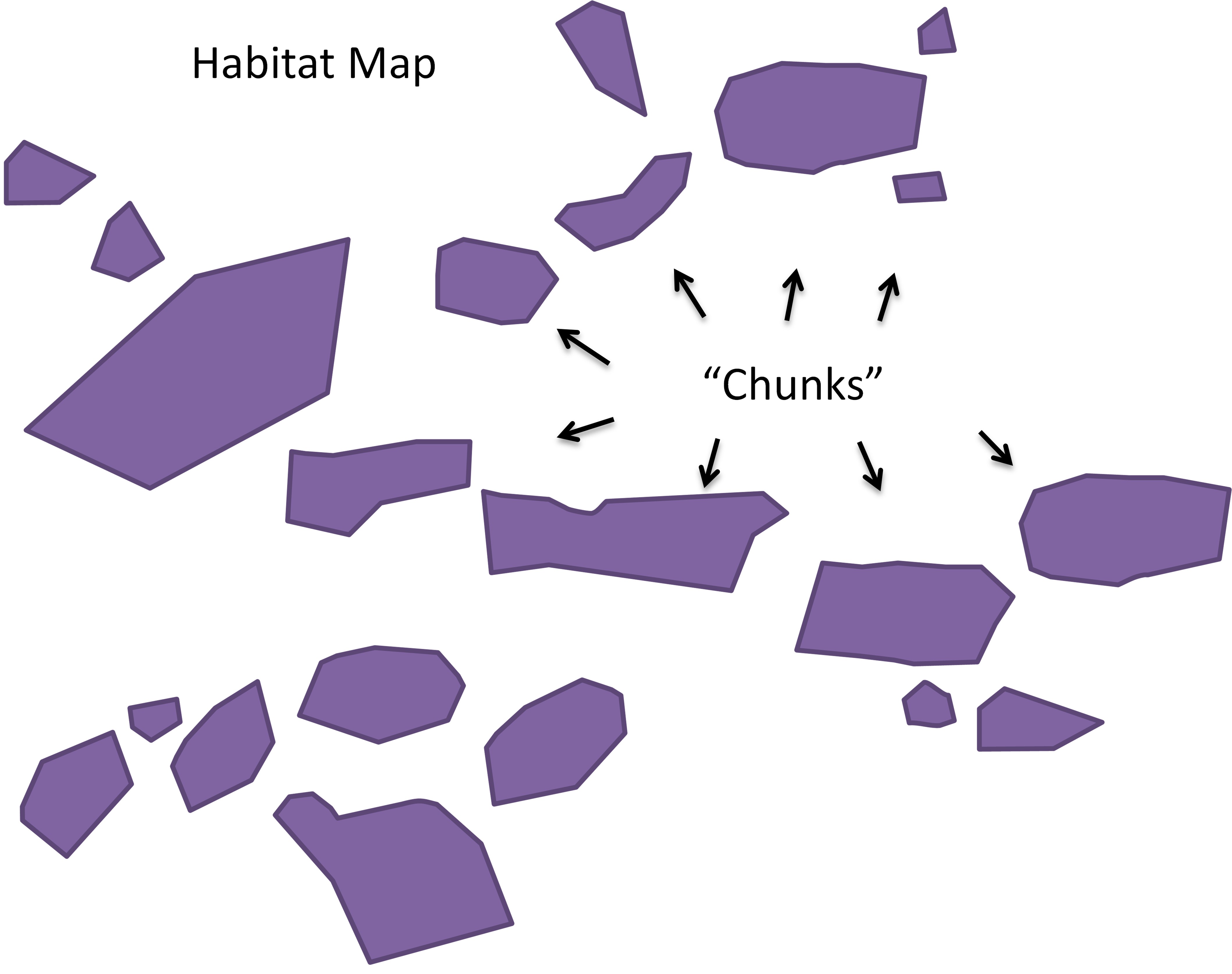
Figure 35. Illustration of a habitat map. Separate pieces of habitat are referred to as “chunks”.
The GeoEFM Patches tool includes three connectivity methods. The physical connectivity method has options for identifying chunks based on connected edge or connected point. The nearest neighbor and buffer methods include cells in chunks based on connected points.
Chunks separated by less than or equal to the user-defined proximity thresholds in the nearest neighbor and buffer methods are grouped into “neighborhoods” (Figure 36). If a chunk is separated by more than the threshold distance in all directions, it is placed in its own neighborhood. Neighborhoods are not used for the physical connectivity method because that method assumes chunks that are physically disconnected do not interact ecologically.
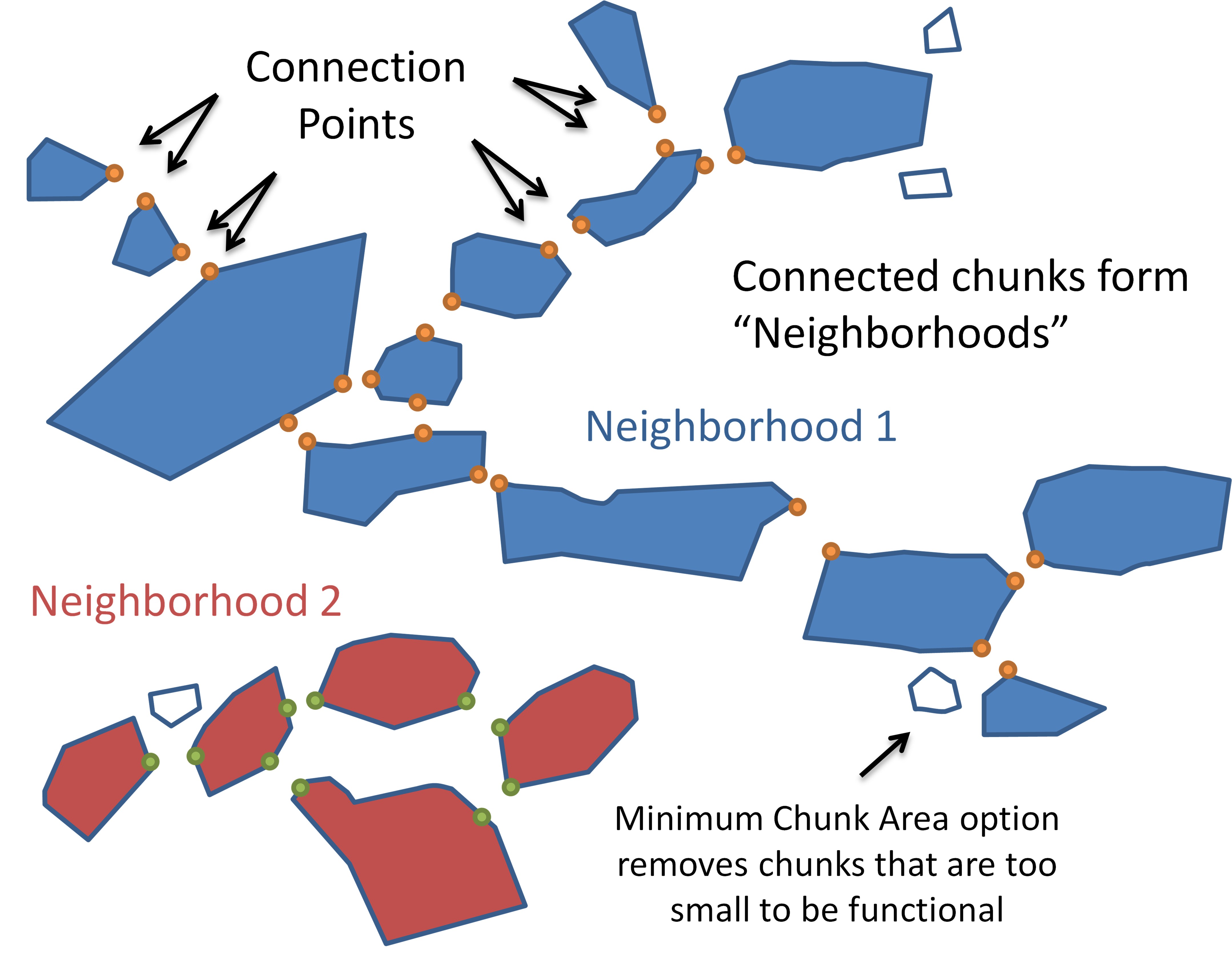
Figure 36. Chunks with areas greater than or equal to the minimum chunk area (user specified and optional) and that are spaced tightly enough to act together ecologically are grouped into “neighborhoods”.
Each neighborhood is assessed separately to split habitat into “patches”, each of which would be a unit of ecological importance such as the amount of habitat needed to support an individual, or habitat for a pack of individuals, or habitat for a nesting site. Being in a neighborhood does not indicate whether there is enough habitat to create a patch, it simply means that the collection of chunks are spaced tightly enough to act together to potentially support one or more patches.
Patch results can be summarized and plotted for areas of interest known as Search Polygons.
Search polygon layers can be created, adopted from other views, or populated with polygons from existing layers. Figure 37 shows the process for creating a new search polygon layer entitled Demo_Search_Polygons through the Patches – Create Search Polygon Layer menu option and then drawing search polygons through the Trace and Split tools in the Manage Search Polygons interface. There is no known limit to the number of search polygons that GeoEFM can consider. Also, search polygons do not need to intersect with or encompass the habitat being considered.
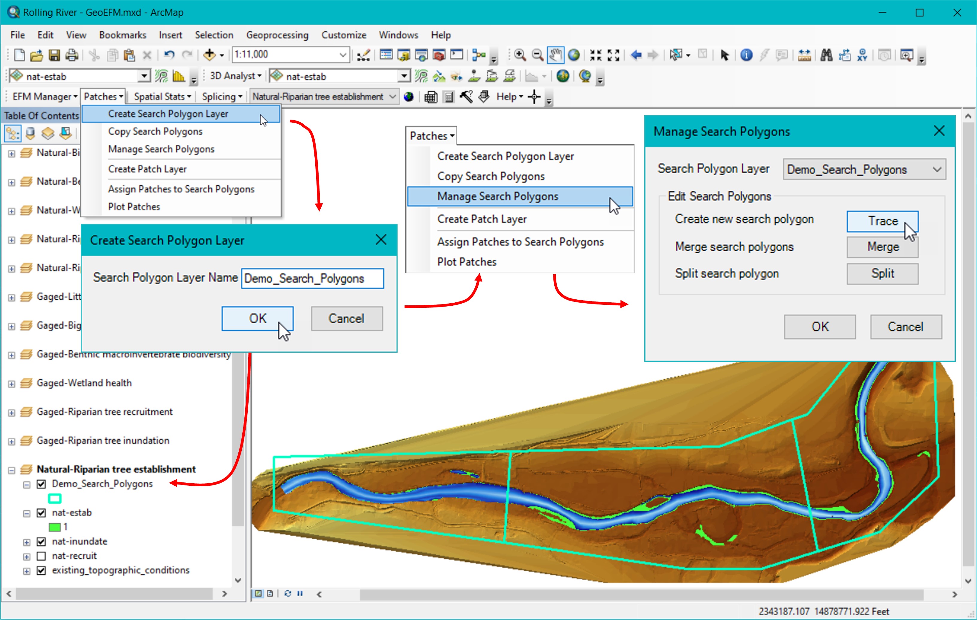
Figure 37. Creating and managing a search polygon layer for use in habitat connectivity analyses.
Once search polygons are established, the next step is to create a “patch raster”, which is simply a raster data set whose data has been split into separate habitat areas known herein as “patches”. For the Physical method a patch is defined by areas that share either a Connected Edge or a Connected Point.
Currently, connectivity can be assessed only for raster datasets.