Case Study: Estimating Benefit of a Proposed FWS for an Urban Watershed

Objective of Hydrologic Engineering Study

A large city in the southeastern United States recently has experienced significant flooding in dense urban watersheds, as illustrated in the following image. Local newspapers described floods of 1995 and 1997 as having "deadly force". Flood insurance claims for the 1995 event totaled $4 million, and an additional $1 million was issued as loans to repair damaged property.

The 1997 flood caused $60 million in damage and took three lives. Total rainfall in the area ranged from 3.87 to 9.37 inches in the 1995 event, and rainfall depths of as much as 11.40 inches in 24 hours were reported in the 1997 event. High water marks indicated that water levels increased by as much as twenty feet in some locations.

Citizens asked USACE to assist with planning, designing, and implementing damage reduction measures. Structural measures, such as those described in the Flood-Loss Reduction Studies, are proposed and will be evaluated. However, for completeness, and to offer some relief in portions of the watershed for which structural measures may not be justified, USACE planners will consider flood warning.

Decision Required

A FWS design has been proposed by a flood-warning specialist. The reconnaissance-level design includes preliminary details of all components shown in the Components of Flood Response and Emergency Preparedness System illustration. To permit comparison of the proposed FWS with other damage-reduction alternatives and to determine if the federal government should move ahead with more detailed design of the FWS, the economic benefit must be assessed. To do so, USACE planners will use the Day curve, and for this, they must determine the warning time in the watershed, without and with the proposed FWS.

As no system exists currently, the expected warning time without the FWS project is effectively zero. The warning time with the FWS will be computed as potential warning time less the detection and notification times. The response and notification times have been estimated as a part of the design, based upon the expected performance of the system components. Thus, the missing components are the recognition and maximum potential warning times. With these times, the warning time will be calculated as the maximum potential warning time less the recognition time.

Watershed Description

One of the critical watersheds for which the FWS will provide benefit is a 4.7 square mile watershed. The watershed is located in a heavily urbanized portion of the city. It has been developed primarily for residential and commercial uses. Several large apartment complexes and homes are adjacent to the channels.

Physical characteristics of the watershed were gathered from the best available topographic data. The watershed is relatively flat with a slope of 0.003. The length of the longest watercourse is 3.76 miles. The length to the centroid is 1.79 miles. The percentage of impervious area is approximately 90 percent.

Procedure for Estimating Warning Time

The maximum potential warning times varies from storm to storm and location to location in a watershed. For example, if damageable property in the watershed is near the outlet, and if a short duration thunderstorm is centered near the outlet, the maximum potential warning time will be small. On the other hand, if the storm is centered at the far extent of the watershed or if a forecast of the precipitation is available before it actually occurs (a quantitative precipitation forecast), the maximum potential warning time for this same location will be greater.

Likewise, the watershed state plays a role in determining the maximum potential warning time. If the watershed soils are saturated, the time between precipitation and runoff is less than if the watershed soils are dry. Accordingly, for this study, the analyst decided to compute an expected warning time for each protected site, as follows:

$//<![CDATA[ \begin{array}{l}\big(5\big) \hspace{5cm} E[T_{w}]= \int_{}^{}T_{w} \big(p\big)dp\end{array} //]]>$

where:

E[T_w] = the expected value of warning time
P = AEP of the event considered
T_w(p) = the warning time for an event with specified AEP

The actual value will be computed with the following numerical approximation:

$//<![CDATA[ \begin{array}{l}\big(6\big) \hspace{5cm} E[T_{W}]= \sum_{}^{}T_{W} \big(p_{i}\big) \Delta p_{i}\end{array} //]]>$

where:

p_i = AEP of event i
T_w(p_i) = the warning time for event i
Δp_i = range of AEP represented by the event

Storm events for this analysis are defined by frequency-based hypothetical storms, as described in the Flood Frequency Studies. With this procedure, the analyst will consider the system performance for the entire range of possible events.

The following image illustrates how the warning time will be computed for each event. First, the analyst used the entire rainfall hyetograph with HEC-HMS to compute a "true" runoff hydrograph, as shown by the solid line. This is the runoff that will occur when the entire rainfall event has occurred. The time that passes between the onset of the rainfall and the exceedance of the threshold is the maximum potential warning time. T_wp, as shown.

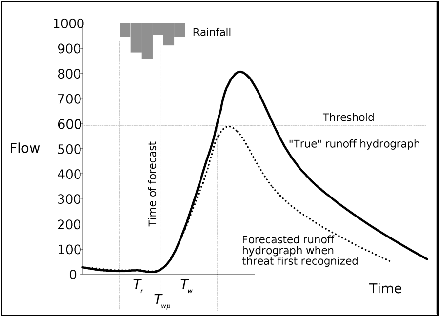
The question that must be answered is this: If the FWS is implemented, when will the system operators be able to detect or forecast that exceedance? That is, what is T_r in the previous figure - the time that passes before the threshold exceedance can be detected (recognition time)? Without the FWS, T_r will approach T_wp, and little or no time will remain for notification and action. The maximum mitigation time, T_w, is then the difference between T_wp and T_r.

To estimate T_r and T_wp for each location in the watershed for which warnings are to be issued, the analyst did the following:

1. Identified the flow threshold at the site, using topographic information, elevation data for vulnerable structures and infrastructure, and simple channel models.
2. Selected a time interval, ΔT, to represent the likely interval between successive forecasts or examination of data for identifying a threat with the FWS. With an ALERT system, data constantly are collected, transmitted, received, and analyzed. For simplicity in the analysis, the analyst used ΔT of thirty minutes and interpolated as necessary.
3. Set up an HEC-HMS model of the watershed, as described below.
4. Ran HEC-HMS for each of the selected frequency-based storms. For each storm, the program was run recursively, using progressively more rainfall data in each run. For example, in the first run with the 0.01 AEP rainfall event, only sixty minutes of the storm data were used. With these data, a hydrograph was computed and examined to determine if exceedance of the threshold would be predicted. If not, thirty minutes of additional data were added, and the computations repeated. When exceedance of the threshold is detected, this defines the earliest detection time for each frequency storm. (Some interpolation was used.) For simplicity, the time of the computation in each case is referred to herein as the Time Of Forecast (TOF). The difference in time from the start of the precipitation event to the TOF where an exceedance was detected is T_r.
5. This computation scheme simulates the gradual formation of a storm, observation of the data over time, and attempted detection of the flood event.
6. Ran HEC-HMS for each of the selected frequency-based storm using the entire precipitation event. The difference in time from the start of the precipitation event to the exceedance of the threshold is T_wp.
7. After finding the detection time and maximum potential warning time for each frequency-based event, computed the expected values, using Equation 2.

Model Selection and Fitting

The analyst hoped to use HEC-HMS for computing runoff from the rainfall. However, the analyst found that model selection for assessment of the FWS benefit presented an interesting challenge. The goal of the study was to determine if a federal investment in developing a FWS was justified. The procedure for estimating the benefit requires an estimate of maximum warning time. Estimating the maximum warning time, as proposed above, requires a model of the watershed. However, developing such a detailed, well-calibrated model of the watershed requires a significant effort, which will not be justified if no federal interest exists. Accordingly, the analyst here developed a simple HEC-HMS model, using regional estimates of parameters. The SCS unit graph transform was used, with lag estimated from an empirical relationship. The initial and constant-rate loss method was selected, and the initial condition and constant-rate loss parameter were estimated with predictors similar to those described in the Urban Flooding Studies. Rainfall DDF functions were defined by referring to appropriate publications from NWS.

Application

The analyst reviewed available topographic information, channel models, and structure data and determined that the threshold for the downstream location in the first watershed of interest is 1,100 cfs. If the discharge rate exceeds this, water will spill from the channel and threaten life and property. Thus a warning would be issued. The goal of the HEC-HMS application is to determine how far in advance a warning of exceedance can be issued.

To identify the detection and maximum potential warning times, the analyst created an HEC-HMS project with a single basin model, but with a large number of meteorologic models. The basin model included representation of all the subbasins, channels, and existing water-control measures. Each meteorologic model defined a portion of a frequency-based hypothetical storm. Eight design storms were used, ranging from the 0.500 AEP event to the 0.002 AEP event. The maximum duration of the storms was six hours. The following figure shows the computed hydrograph for the eight storms, using the rainfall for the entire six-hour duration. Events smaller than the 0.040 AEP event do not exceed the threshold. Column 2 of the following table shows the maximum potential warning time for each of the events: the time between initial precipitation and threshold exceedance.

To complete the runoff analysis as proposed, each of the hypothetical events was analyzed with increasing duration of rainfall data, starting with sixty minutes of data. The analyst increased the duration of data in thirty-minute blocks and computed a runoff hydrograph.

To create the meteorologic models for this, the analyst used HEC-HMS and a combination of HEC-DSSVue (HEC Data Storage System Visual Utility Engine) data management tools. First, the DSS file in which rainfall hyetographs from the total storm are stored was identified. To accomplish this, the analyst used Windows® Explorer to examine the contents of the HEC-HMS project folder. There the USACE analyst found a file with the extension ".dss". In each project, HEC-HMS stores all the computed and input time series for the project, including, in this case, the rainfall hyetograph for the six-hour design storm. Next, the analyst used one of the available tools for manipulating DSS files. In this case, the analyst used DSSUTL (DSS Utility software), and with it created duplicates of the DSS record in which the six-hour storm hyetograph is stored.

Records stored in a DSS file have a unique name (pathname) consisting of six parts. This so-called pathname serves as the primary key in the database, permitting efficient retrieval of records. The parts of the pathname are referred to as the A-Part, B-Part, and so on. Some parts serve a specific purpose. For example, the C-Part identifies the type of data stored in the record, and the E-Part identifies the reporting interval for uniform time series data. The F-Part may be assigned by a user, so the analyst assigned an F-Part unique to the duration of data available to each copy of the rainfall. For example, the sixty-minute sample of the 0.01 AEP event was assigned an F-Part of 01AEP60MIN, while the 300-minute sample for the 0.002 AEP event was assigned an F-Part of 002AEP300MIN. Then the analyst used DSSUTL with an editor compatible with DSS to delete values from the series, shortening each to include just the duration of rainfall required. For example, the final 300 minutes of the six-hour storm was deleted to create the sixty-minute sample, and the final 270 minutes was deleted to create the ninety-minute sample. Eleven such copies were made for each of the eight frequency based storms, for durations from sixty minutes to 360 minutes.

Next, a meteorologic model was created in HEC-HMS for each of the samples. To accomplish this, the analyst identified each shortened sample as a precipitation gage and used the gage to define a hyetograph. While the series are, in fact, not gaged data, they may be used as such for runoff computations with HEC-HMS. (This useful feature also permits computation of runoff from any hypothetical storm types that are not included in HEC-HMS.) To create the precipitation gage time-series, from the Components menu, the analyst clicked Time-Series Data Manager. The Time-Series Data Manager opens; the analyst selects a data type from the Data Type list - Precipitation Gages. To create a precipitation gage, click New, the Create a New Precipitation Gage window will open. Provide a name; click Create, the Create a New Precipitation Gage window closes. In order to add data to the precipitation gage, the analyst opened the precipitation gage Component Editor.

When a new time-series gage is added to a project, the HEC-HMS user has the option to retrieve the values from an existing DSS file or to enter manually the ordinates by typing the data in a table. From the Data Source list the analyst has selected Data Storage System (HEC-DSS) this will allow retrieve of values from an existing DSS file.

The next step for using time-series data in an existing DSS file is to select the DSS file and the correct data record within the file. Click the Open File Chooser, a browser (Select HEC-DSS File) will open, select the appropriate DSS file, click Select. The selected DSS file will now display in the DSS Filename text box. After the correct DSS file has been selected, click Select DSS Pathname , the Select Pathname From HEC-DSS File Editor will open. From the Editor, the list of data records in the selected DSS file is displayed. With this, almost any record from any DSS file to which the analyst has access can be selected and assigned to the gage.

This task of adding a gage and associating data from a DSS file, was repeated to create one gage for each combination of storm and duration. The result was a set of 88 gages for the eight frequency-based storms.

Next, the analyst created a meteorologic model for each of the cases, using the 88 precipitation gages to define the hyetographs. To do so, the analyst created a meteorologic model and selected Specified Hyetograph, as shown in the following figure. In the specified hyetograph Component Editor, the analyst selected from among the 88 precipitation gages.

At last, the preparation for the computations was complete, and the runoff hydrographs could be computed and inspected. To insure that this computation was complete, the analyst used the Simulation Run Manager to "assemble" the simulation runs, using the basin model and control specifications in combination with each of the rainfall events.

The following figure shows the results of the HEC-HMS simulation runs. For each frequency storm, the computed peak with each portion of the six-hour event is plotted. From this, the time at which threshold exceedance (flow greater than 1,100 cfs) would be detected can be identified. For example, with the 0.002 AEP event, exceedance would not be detected with only 150 minutes of rainfall data, but it would be detected with 180 minutes of data; interpolation yields an estimate of 175 minutes as the detection time for that event. The estimated values for all events are shown in Column 3 of the Sample Calculation of Warning Time table. Column 4 of that table shows the maximum mitigation time. The actual mitigation time would be less if time is required for notification and decision making. For example, if twenty minutes is required for notification and decision making, the mitigation time available for the 0.002 AEP event will be only forty minutes. Forty minutes provides little opportunity for property protection, but it is enough time to evacuate, if plans have been made and if the evacuees are well prepared.

Results Processing

The objective of the study, of course, is not to run HEC-HMS to compute hydrographs, so the work required is not complete. Now the analyst must process the results, using Equation 2, to estimate an average warning time with which benefit can be estimated.

At the onset of this computation with Equation 2, the analyst realized that events smaller than the 0.04 AEP event did not exceed the threshold. Including those in the expected value calculation might bias the results, as the warning time would be infinite (no warning would be issued because the threshold was never exceeded). Accordingly, the analyst decided to use conditional probability in the computations, reasoning that the expected value should use only events that exceeded the threshold.

So, by integrating the maximum mitigation time-frequency curve, as directed by Equation 6, and using conditional probability to account for events more frequent than the 0.04 AEP event, the analyst computed expected warning time. For the proposed system, the maximum expected warning time was 55 minutes at the critical location. Based on the system design, the flood-warning specialist optimistically estimates the notification and decision-making time to be twenty minutes. Thus, the actual expected mitigation time is 35 minutes. The resulting damage reduction is slight, but the cost of a local FWS is also relatively small, so a federal interest may exist.