Case Study: Channel Maintenance along Stirling Branch

Watershed Description

Stirling Branch is a tributary of Deer Creek in a developing area in the western United States. The average elevation of the contributing watershed is 1,300 feet. The total watershed area is 1.23 square miles. The watershed has pockets of relatively high-density development. Watershed slopes are relatively steep. The creek channel slopes are on the order of three percent in the upper reaches and about one percent in the lower reaches. The creek crosses several roads in the watershed through culverts, which produce major obstructions to flow.

Development in the watershed has had a significant impact on the stream corridor. As illustrated in the following image's "Current Condition", the channel has been straightened, and the riparian corridor has been altered, with native vegetation removed for the sake of hydraulic efficiency of the channel. The channel has been directed through culverts at the road crossings. A maintenance program was established by the local government to maintain these "clean" channels and to ensure that the culverts were clear.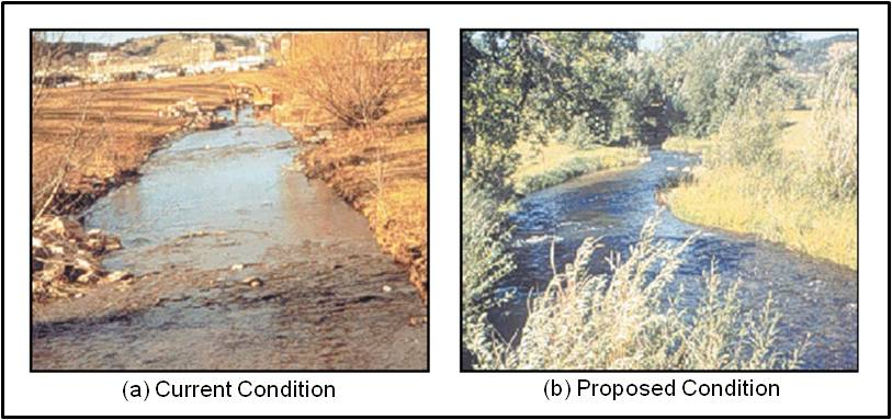

The local government has now reconsidered the wisdom of this channel modification and the maintenance, and has appealed to USACE for technical assistance in restoring the stream. A local environmental group has supported this, suggesting that the channel should be restored to a state similar to that shown in the previous image's "Proposed Condition", with ground-level shrubs and trees of moderate density planted in the stream corridor. USACE environmental specialists have suggested omitting the ground-level shrubs and planting only trees that would be trimmed to keep branches above the 0.01 AEP water surface elevation. However, owners of property adjacent to the stream are not so keen on the restoration. They are concerned that the vegetation in the floodplain will induce flooding, as it obstructs flow. To provide the necessary information to make decisions about the restoration, a hydrologic engineering study with HEC-HMS was undertaken.

Decisions Required and Information Necessary for Decision Making

The decision required is this: which, if any, of the proposed stream restoration projects should be selected for implementation? Much information beyond what can be provided by a hydrologic engineering study is necessary to make this decision. However, in this case, the analyst was called upon to provide the flows in and downstream of the restored reach for the 0.50 AEP, 0.10 AEP, and 0.01 AEP events. The 0.50 AEP (2-year) peak flow is a critical parameter for restoration, as this is the bank full or channel-forming flow in the natural stream system; it will be used for sizing many features of the project. The 0.01 AEP event is used for floodplain-use regulation, and thus is a good indicator of any adverse impact of the restoration: If this flow increases significantly, it is an indication that damage may be incurred downstream. The 0.10 AEP event is an intermediate event, and is often used for design of storm water management facilities. Thus, it provides a benchmark for comparison.

Model Selection

The following figure shows velocity profiles for several vegetation types; in this illustration, all are submerged to some extent. In (a), low vegetation is fully submerged by a higher flow rate. In this case, the velocity is retarded, and the velocity gradient is near zero within the canopy. Above the canopy, the velocity increases approximately logarithmically. In (b), a tree is partially submerged. Lower branches of this tree are trimmed to have less impact on lower flow rates or on the velocity profile at the lower boundary. In (c), trees are combined with lower vegetation. In this case, velocity is retarded by both the undergrowth and the tree branches.

These changes in velocity will alter depths in the channel and discharge rates downstream. While a detailed analysis of this requires a detailed open channel model, the simplified routing methods included in HEC-HMS can provide insight to changes in the discharge rates. Thus, in this case, the critical hydrologic engineering component is the channel routing method.

With the relatively steep stream and fast rising hydrographs from the small contributing watershed, the Muskingum-Cunge routing method is an appropriate choice for this analysis. This method can conveniently reflect changes to the channel cross section and changes to the channel roughness due to the vegetation.

Of course, the analyst also needed to develop a basin model to compute the inflow hydrographs - the boundary conditions for the channel routing models. For this, the watershed was subdivided into six subbasins (primarily for convenience of modeling the channels). For each, the SCS CN method was selected for runoff volume computation and the SCS UH method was used for transforming rainfall excess to runoff.

Model Fitting and Verification

Subbasin models. The subbasins were ungaged, so no direct calibration was possible to estimate parameters. Instead, the analyst found the average CN for each subbasin using GIS (geographic information system) tools with coverages of land use and soil type.

The SCS UH lag was estimated for each subbasin as sixty percent of the time of concentration for each subbasin, following SCS recommendations. The time of concentration for each subbasin was estimated with procedures suggested by the SCS (SCS, 1971, 1986). Based upon experience with gaged watersheds in the region, this estimate has been shown to yield reasonable results for those watersheds.

Routing models. The restoration alternatives which were proposed correspond to scenarios illustrated in (b) and (c) of the previous figure. To represent these, the analyst selected the Muskingum-Cunge routing method and entered geometric data appropriate for each case, as shown below.

The existing, without-project-condition cross sections were surveyed at selected locations. Roughness values for the main channel and both overbanks were estimated for the without-project condition after a field investigation. Photographs of the channel were taken and compared with those in Barnes (1967) to select the Manning's n values.

Channel cross sections were proposed for the restoration alternatives by the study team's plan formulators. Modified Manning's n values for the alternatives were estimated using Fischenich's equation (1996) for flow resistance in channels with non-submersed vegetation:

$//<![CDATA[ \begin{array}{l}\big(7\big) \hspace{5cm} n = k_{n}R^{2/3}\begin{bmatrix}\frac{C_{d}Veg_{d}}{2g} \end{bmatrix} ^{1/2}\end{array} //]]>$

 where:

C_d = coefficient to account for drag characteristics of vegetation;
Veg_d = vegetation density; and
g = gravitational constant

Vegetation density is defined as:

$//<![CDATA[ \begin{array}{l}\big(8\big) \hspace{5cm} Veg_{d}= \frac{ \sum_{}^{} A_{i} }{AL}\end{array} //]]>$

where:

A_i = area of vegetation below water surface, projected onto a plane perpendicular to direction of flow
A = cross-sectional area
L = characteristic length

Flippin-Dudley (1998) suggests that C_d can be estimated as:

$//<![CDATA[ \begin{array}{l}\big(9\big) \hspace{5cm} C_{d} = 2.1 \big(VR\big)^{-1.1}\ with\ debris\ present\ and\ leaves\ absent\ from\ trees\ and\ shrubs;\end{array} //]]>$

$//<![CDATA[ \begin{array}{l}\big(10\big) \hspace{5cm} C_{d} = 0.28 \big(VR\big)^{-1.1}\ with\ debris\ removed\ and\ leaves\ present.\end{array} //]]>$

The analyst used these relationships, finding and using the worst case (greatest n value) for each stream reach.

Boundary Conditions and Initial Conditions

Hypothetical frequency-based storms were defined, as illustrated in earlier chapters. The SCS CN method defines, by default, an initial loss that is a function of the CN. This was used here. While the analyst's intuition was that the average initial loss for the 0.50 AEP event would likely be much greater than that for the 0.01 AEP event, the analyst realized that this parameter likely would have little impact on the decision making. The goal of the analysis was to compare the impact of the restoration alternatives, not to complete a detailed flood-damage analysis.

Application

An HEC-HMS project was developed for the analysis as follows:

1. A single control specification was developed, with a time interval appropriate for the subbasin with the shortest time of concentration. The minimum time of concentration was 28 minutes, so a time interval of four minutes was selected.
2. A meteorologic model was prepared for each of the three hypothetical rainfall events. A 24-hour storm was used. For this small watershed, a shorter duration storm would likely be adequate for definition of the peaks. However, many design studies in the region have been completed with 24-hour storms, so for consistency, that was used here.
3. A basin model was created for each of the three cases of interest: no restoration; restoration with trimmed trees in the floodplain; and restoration with trees and shrubs. The subbasin runoff elements were identical in these three basin models, but the routing models varied in each to represent the differences in channel cross section and vegetation in the floodplain. The basin schematic is shown below.
4. The analyst defined nine simulation runs, combining the three meteorologic models with the three basin models. Peak flows at the watershed outlet are shown in the table below.

Clearly the restoration has an impact on the downstream peaks. The greater the vegetation in the channel, the more the peak flow was attenuated, thus resulting in a lower peak flow. However, the peak stage was likely increased and needs to be investigated with a hydraulic model. HEC-RAS could be used for this analysis.

Additional Analysis

The analysis described here provides only part of the hydrologic engineering information required for evaluation of the restoration alternatives. It does not provide information about depths of flooding or velocities. That information was developed for this study using HEC-RAS. The HEC-HMS and HEC-RAS models developed by the analyst shared cross-section geometric data and estimates of Manning's n. Thus, the models provided quick-and-dirty checks of reasonableness: The HEC-RAS model provided velocity estimates, with which travel time could be computed. The computed translation of hydrographs in the channels was compared with this, and some fine-tuning was done.

If a more detailed analysis is warranted, the channel routing in HEC-HMS may be substituted with an unsteady flow hydraulics model such as HEC-RAS. HEC-HMS could be used to compute the local inflows to the channels, and then using DSS, the flows can be input to HEC-RAS. To do this, additional channel geometry and refinements in channel parameters may be needed. During this more detailed analysis, natural channel tendencies, from a geomorphic standpoint, will need to be examined. For example, water velocities may erode the vegetation and tend to straighten the channel.