Download PDF
Download page Applying the Linear Reservoir Baseflow Method.
Applying the Linear Reservoir Baseflow Method
Last Modified: 2025-01-29 17:47:34.44
Overview
In this tutorial you will apply the HEC-HMS linear reservoir baseflow method to a modeling application. Initial parameter estimates will be determined, and the model will be calibrated through trial and error.
Software Version
HEC-HMS version 4.13-beta.4 was used to create this example. You can open the example project with HEC-HMS 4.13 or a newer version.
Project Files
Download the Initial project files here:
Note: The initial project file is the same for the Constant Monthly, Recession, and Linear Reservoir Baseflow tutorials. If you are completing all three tutorials, the files only need to be downloaded once.
Initial Parameter Estimates
- Open the Punxsutawney project and then open the Mahoning Creek Linear Res Basin Model.
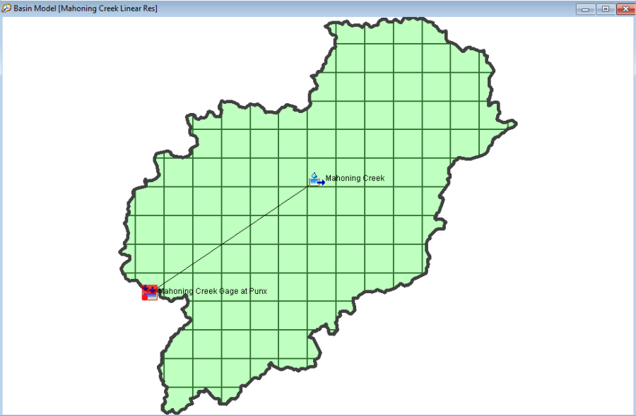
- Select the Sept2018_LinearReservoir simulation run from the Compute toolbar,
 . Press the Compute All Elements button,
  , to run the simulation.
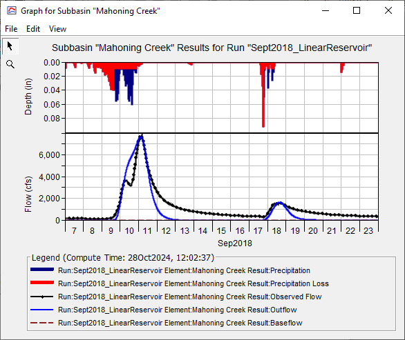
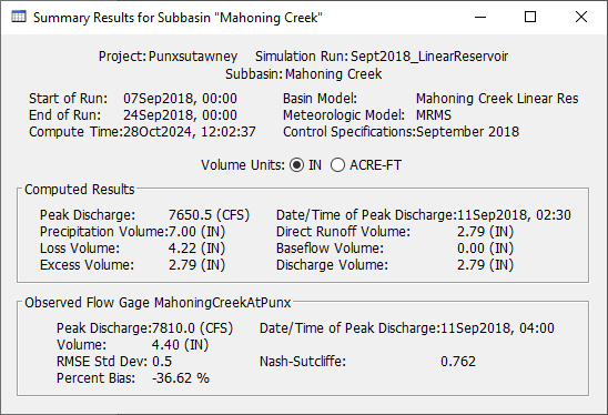
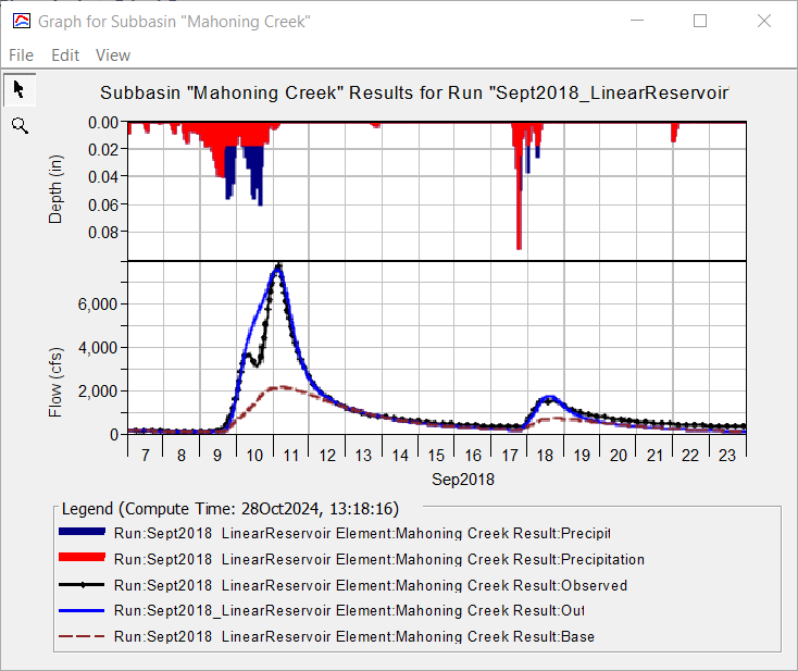
 - View the result graph and summary table for the Mahoning Creek subbasin element. Notice the computed flow does a good job matching the peak observed flow, but the interflow and baseflow portions of the computed hydrograph do not match observed flow. The summary table shows a large difference in observed and computed runoff volume (4.40 inches vs. 2.79 inches). Leave the summary table and plot open so you can see results change as you add baseflow and modify baseflow parameters.
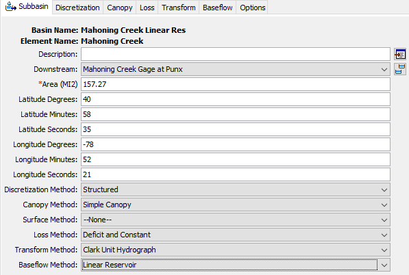
- Open the Component Editor for the Mahoning Creek subbasin element. Change the Baseflow Method from None to Linear Reservoir.
- Go to the Baseflow tab to enter Linear Reservoir parameters.
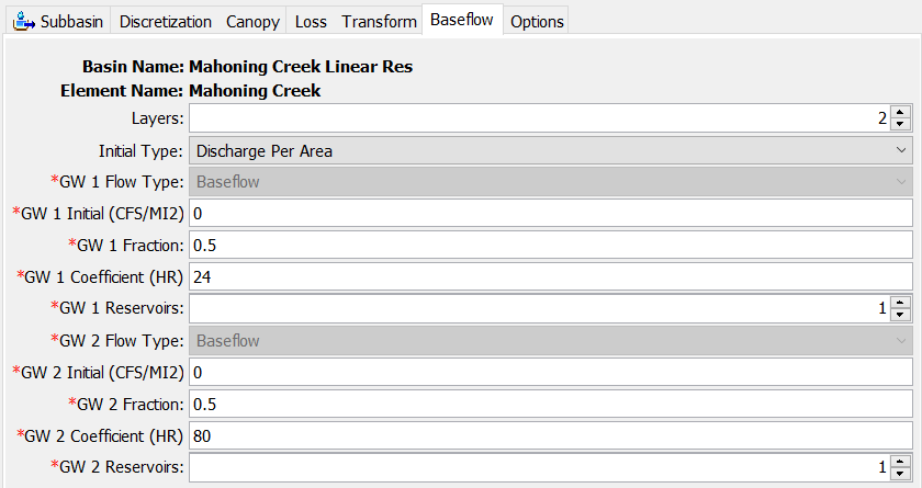
- Select 2 Layers. We will use the Groundwater (GW) 1 layer to model faster responding interflow and GW 2 to model slower responding baseflow.
- Change the Initial Type to Discharge Per Area. Enter 0 CFS/MI2 for both GW 1 Initial and GW 2 Initial.
- Set the GW 1 Fraction to 0.5 and the GW 2 Fraction to 0.5. Initially, we are dividing all infiltrated precipitation equally between both GW 1 and GW 2 reservoirs.
- Set the GW 1 Coefficient so that it is 3 times larger than the Clark Storage Coefficient (8 hours * 3 = 24 hours). Set the GW 2 Coefficient so that it is 10 times larger than the Clark Storage Coefficient (8 hours * 10 = 80 hours).
- Leave the number of GW 1 Reservoir and GW 2 Steps at 1.
- Re-run the simulation and look at the results plot and summary table. Notice baseflow in the plot and how the addition of baseflow to direct runoff results in an increase in the simulated peak flow. The total runoff volume increased as well. The direct runoff is 2.79 inches and the baseflow is 1.46 inches. Water that infiltrates due to the constant loss rate now contributes to runoff from the subbasin element.


Calibrate the Model
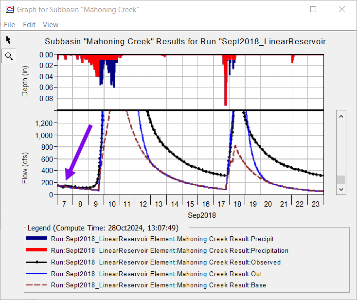
- The easiest baseflow parameter modification to make is to set the initial baseflow at the beginning of the simulation so that the simulated results match observed flow. For most applications, only use GW 2 to match observed flow at the beginning of the simulation. GW 1 typically represents faster responding interflow and leaves a watershed soon after a flood event. GW 2 typically represents the slower responding baseflow and is usually the only type of stream flow when there has been a longer period since a precipitation-runoff event. If you zoom into the plot, you will see the observed flow value is approximately 160 cfs at 00:00 on September 7, 2018. The drainage area for the subbasin is 157.27 square miles; therefore, the initial GW 2 flow can be set by dividing 160 cfs by 157.27 square miles, which is approximately 1 CFS/MI2. Change the GW 2 Initial value from 0 to 1 CFS/MI2. Rerun the simulation. You should notice a close match in observed and computed flow at the beginning of the simulation.
The next step is to identify the parameters to adjust and understand their impact on computed results. Since the Linear Reservoir baseflow method conserves mass, the infiltration rate should be adjusted along with the baseflow parameters when improving model results. - Change the Constant Loss Rate from 0.038 in/hr to 0.08 in/hr by clicking on the Loss tab. Re-run the simulation. Notice how the simulated peak flow is reduced while the baseflow hydrograph increased (less surface runoff and more baseflow when increasing the constant loss rate).
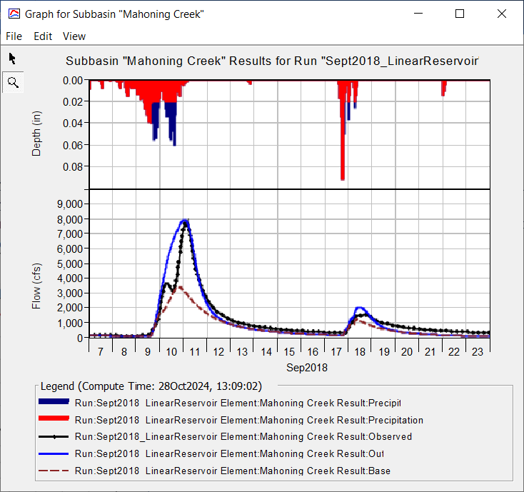
- In the figure above, notice how the baseflow hydrograph (dashed purple line) peaks on September 10 while the total flow hydrograph (solid blue line) peaks on September 11. Baseflow should occur after direct runoff. Increasing the GW 1 Coefficient will shift the time of peak flow for the baseflow hydrograph. Increasing the number of linear reservoirs has a more pronounced shift in the timing of the baseflow hydrograph. Increase the GW 1 Reservoirs from 1 to 2. Do not modify the GW 1 Coefficient. Re-run the simulation and look at the results plot. The timing of the baseflow hydrograph looks better, and the shape of the recession curve matches the observed flow much better too.

In the Results tab, individual Baseflow Layer time series results can be previewed. Viewing individual baseflow layers allows users to see how parameter changes impact the flow and can assist with the calibration process. Holding the Ctrl button allows you to select and plot multiple time series results.

- The GW 1 and GW 2 Fractions can be used to shift infiltrated water between groundwater layers. Change the GW 1 Fraction to 0.1 and the GW 2 Fraction to 0.9. Re-run the simulation and look at the results plot. Overall, the results are not improved with the change. The simulated peak flow is reduced, while there is slight improvement on the baseflow only portion of the hydrograph. More infiltrated water goes to the slower responding GW 2 linear reservoir (90 percent to the GW 2 reservoir vs. 10 percent going to the GW 1 linear reservoir). The GW 1 and 2 Fractions can be used to remove water to a deep, non-contributing aquifer, if needed. The GW Fractions do not have to sum to a value of 1. If the Fractions do not sum to 1, then the difference (1 - sum of the GW Fractions) is lost to a deep aquifer and will not contribute to runoff from the subbasin.
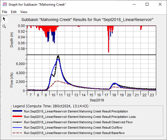
- Continue adjusting the Constant Loss Rate, and the GW 1 and 2 Fractions, Coefficients, and number of Steps to calibrate the model. Record your Nash-Sutcliffe score as you adjust model parameters.
Project Files
Download the Final project files here:
Note: The final project file is the same for the Constant Monthly, Recession, and Linear Reservoir Baseflow tutorials. If you are completing all three tutorials, the files only need to be downloaded once.
Questions:
Question 1: Why should the linear reservoir groundwater coefficients be related to the Clark storage coefficient?
It is not necessary to link the linear reservoir groundwater coefficients to the Clark storage coefficient. However, similar processes that impact storage, attenuation, and timing of surface water impacts the response of interflow and baseflow. Interflow and baseflow happen throughout the watershed. Infiltrated water moves through the soil and then exfiltrates into a small channel. Once in the channel network, water flows in the stream network to the subbasin outlet. The path water takes after it exfiltrates into a channel is similar to the path direct runoff takes. The difference is that groundwater flow / baseflow spends a portion of the travel time in the soil, which is accounted for by increasing the baseflow coefficient or adding multiple linear reservoirs (steps). Another reason to ratio unit hydrograph and baseflow storage coefficients is to reduce the complexity of parameterizing a basin model with many subbasins. Using ratios is a quick way to parameterize a model while linking parameters that are conceptually similar.
Question 2: What were your final loss and groundwater parameters? What was the Nash-Sutcliffe score for the calibrated model?
The final Constant Loss Rate was set to 0.07 in/hr. The following figure shows the final Linear Reservoir Baseflow parameters. The Nash-Sutcliffe score was 0.932.


Continue to Applying the Recession Baseflow Method
