Download PDF
Download page Task 1: Quick Debris Yield Modeling based on Field Data (with New Debris Volume Conversion to Mass with Unit Weight/Density).
Task 1: Quick Debris Yield Modeling based on Field Data (with New Debris Volume Conversion to Mass with Unit Weight/Density)
Last Modified: 2023-10-24 06:38:25.418
Overview
This workshop illustrates steps to develop a basic HEC-HMS debris yield model from scratch using existing field data. This workshop focuses on developing a debris yield model quickly. The outputs from the model will only produce sediment yield. This is relevant for emergency response situations where the modeler is expected to produce a quick, approximate estimate of accumulated sediment/debris yield based on given field data from the burned watershed. In this workshop, you will summarize the field data and choose appropriate input parameters for the debris yield simulation. More information on the debris yield parameters is contained in the User's manual.
Download Initial Project Files: Task 1 inputs.xlsx
Data acquisition and field investigation are required to estimate input parameters (using rainfall data, topographic maps, soil burn severity map, field soil sample, etc.) Field data also requires collecting soil samples to generate a gradation curve. The following data was collected for you using a precipitation gage, 30-meter digital elevation model, and soil burn severity map. This gradation curve was estimated based on a published data set since a field soil sample was not available. Methods for developing gradation curves are described here.
| Debris Basin | Area (KM2) | Longest Flowpath Length (KM) | Basin Relief (M) | Relief Ratio (M/KM) | Burn Date | Burn % | Burned Area(KM2) | Rainfall | Debris Yield Simulation Period |
|---|---|---|---|---|---|---|---|---|---|
| Brand DB | 2.63 | 2.87 | 620.47 | 216.19 | Sep 02 2002 | 90 | 2.36 | Forecasted Rainfall (Generated based on Childs Canyon Gage data for this workshop) | 16Mar2003, 00:00 - 16Mar2003, 04:00 |
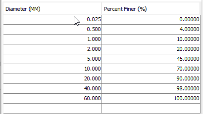
Gradation Curve
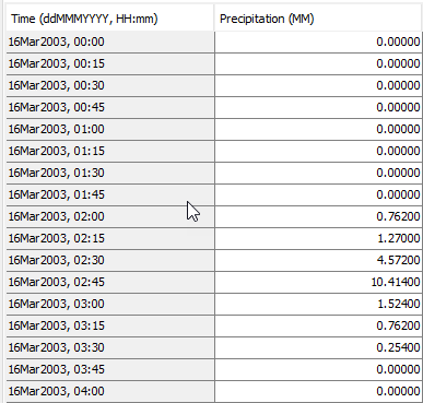
Forecasted Rainfall Amounts (16 Mar 2003 00:00 - 16 Mar 2003 04:00)
Develop the Model
- Create a new HEC-HMS project with HEC-HMS version 4.12 beta 1 or greater by selecting File | New.
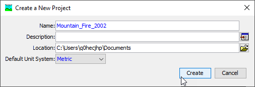
- Name the project Mountain_Fire_2002
- Set the proper project Location.
- Set the Default Unit System to Metric.
- Create a new basin model by selecting Components | Create Component | Basin Model
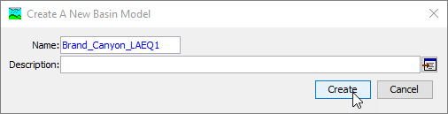
- Name the basin model Brand_Canyon_LAEQ1
- Name the basin model Brand_Canyon_LAEQ1
- Select the Basin Models folder to expand the Watershed Explorer.
- Select Brand_Canyon_LAEQ1 Basin Model.
- Click the subbasin creation tool icon
 in the components toolbar.
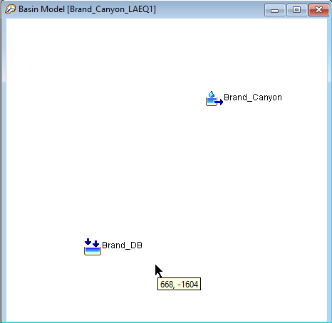
 - Click on the basin map to create a subbasin element and name the subbasin element Brand_Canyon.
- Switch to the sink creation tool icon
 in the components toolbar.
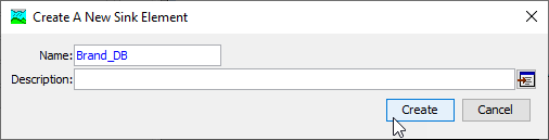
 - Click on the basin map to create a sink element and name the sink element Brand_DB.
- The elements should be placed as shown in the figure below.
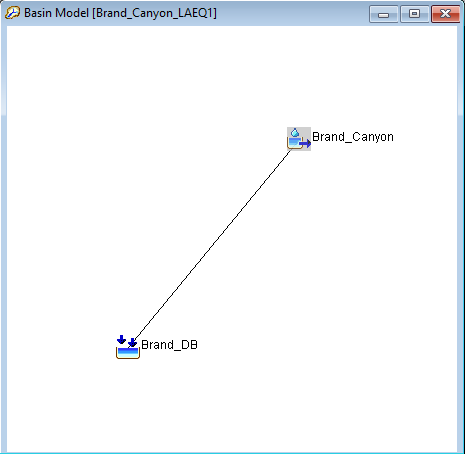
- Connect the elements into a hydrologic network as shown in the figure below. Right click on Brand_Canyon subbasin element and select the Connect Downstream option. Use the mouse to identify the sink element Brand_DB that should be downstream. A connection line is drawn to show the elements are connected
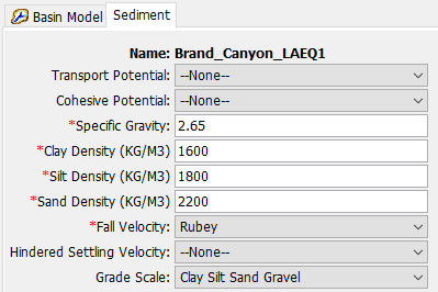
- Select the Basin Model (Brand_Canyon_LAEQ1) in the Watershed Explorer and then select Yes for the Sediment option in the Basin Model Tab as shown below.

- Updated sediment Density as show below on the Sediment tab. This values were assumed based on the literature (1500-2200 KG/M3) for debris mixture densities.
- Select the subbasin element Brand_Canyon.
- Select the Subbasin Tab.
- Enter the Area (2.6263 Km2) and select None for all of methods. Select LA Debris Method EQ1 for the Erosion Method as shown below.
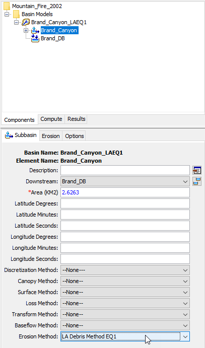
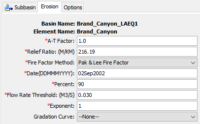
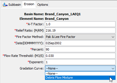
- The LA Debris Yield Equation 1 contains four parameters. The Pak & Lee Fire Factor method adds another two parameters. These parameters can be estimated from the watershed terrain, burn severity maps, and field samples. The Flow Rate Threshold and Exponent are parameters added to HEC-HMS to identify storms that generate debris/sediment and to distribute a storm debris/sediment amount into a time-series, sedigraph. Select the Erosion Tab and populate initial parameters values based on the given data provided below. Erosion parameters are described in the User's manual.
- A-T Factor: 1.0 (Default Value)
- Relief Ratio (M/KM): 216.19 (from Table above)
- Fire Factor Method: Pak & Lee Fire Factor (Select this option for this case)
- Date (DDMMMYYYY): 02Sep2002 (from Table above)
- Percent: 90 (from Table above)
- Flow Rate Thresholds (M3/S): 0.030 (Default Value)
- Exponent: 1 (Standard Value)
Question 1: What parameter from LA Equation 1 is determined and computed for you in HEC-HMS?

The maximum 1-hour precipitation. This is determined for you from the precipitation gage. You do not need to enter this value.
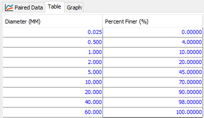
- Prepare a Gradation Curve based on the given information.
- Click Components | Paired Data Manager.
- Select Data Type: Diameter-Percentage Functions.
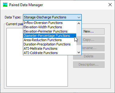
- Click New.
- Name the gradation curve Debris Flow Mixture.
- Click Create.
- Select the newly added gradation curve in the Watershed Explorer.
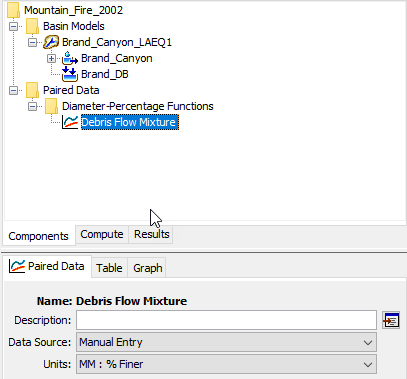
- Select the Paired Data tab.
- Select Data Source: Manual Entry.
- Select Unit: MM : %Finer.
- Select the Table tab and enter the values for the gradation curve as shown in below. You can copy the values from the provided spreadsheet file.
- Go back to the Erosion Tab for the Brand_Canyon subbasin and select the Debris Flow Mixture Gradation Curve.
- Create a new Meteorologic Model.
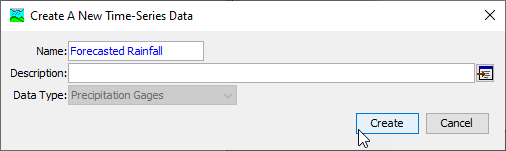
- Create a new precipitation gage. Go to the Components | Time-Series Data Manager menu option. Under Data Type, select Precipitation Gages. In the manager window, press the New button.
- In the new gage window, change the default name to Forecasted Rainfall. Press the Create button.
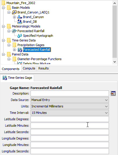
- In the Watershed Explorer, click on the new gage you just created. The units should be set to Incremental Millimeters and the Time Interval set to 15 Minutes.
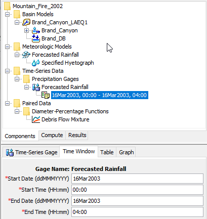
- In the Watershed Explorer, click the + button on the Forecasted Rainfall gage to expand the tree and see a list of time windows. Select the default time window to open the Component Editor. In the Component Editor, change start date to 16Mar2003, the start time to 00:00, the end date to 16Mar2003, and the end time to 04:00.
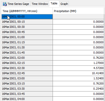
- Click on the Table tab and enter the Precipitation values as shown below. You can copy the values from the provided spreadsheet file.
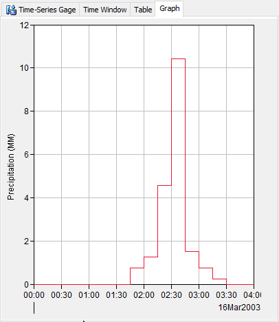
- Click on the Graph tab in the Component Editor to see the data.
Question 2: Where can you go to get forecasted rainfall for a region?Forecast rainfall can be obtained from your River Forecast Center (RFC). In California, the California Nevada River Forecast Center (CNRFC) provides forecasted rainfall at 6-hr or 24-hr time steps.
- Select the Components | Meteorologic Model Manager menu option. Press the New button to create a new Meteorologic Model and name it Forecasted Rainfall.
- Click on the new Meteorologic Model Forecasted Rainfall you just created and populate the Meteorologic Model parameters as shown below.
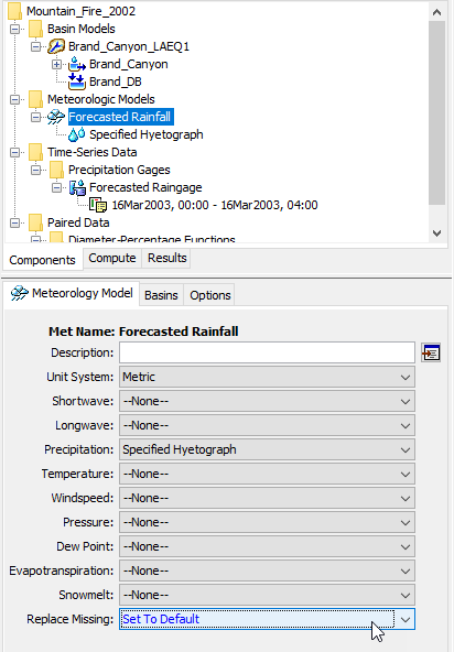
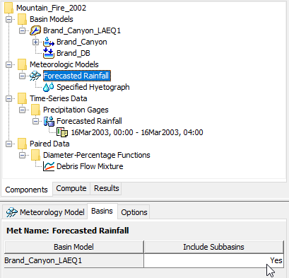
- Select to the Basins tab and select Yes in the Include Subbasins column (we need to link precipitation gages to subbasins elements in the Brand_Canyon_LAEQ1 basin model).
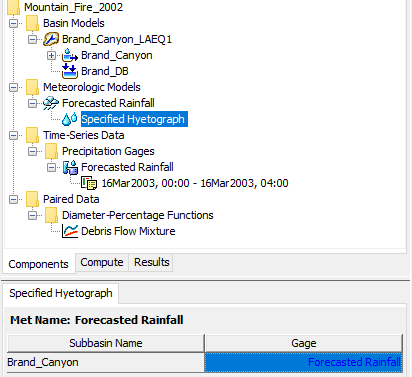
- In the Specified Hyetograph node, select the newly-created precipitation gage Forecasted Rainfall in the Gage column.
- Create a new Control Specifications.
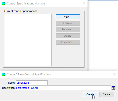
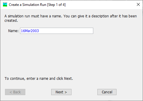
- Select the Components | Control Specifications Manager menu option. Press the New button to create a new Control Specifications.
- Change the name to 16Mar2003 and enter a description of Forecasted Rainfall. Press the Create button.
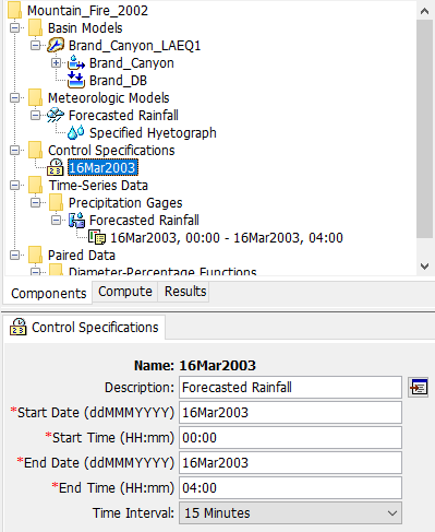
In the Watershed Explorer, click on the control specifications you just created. Enter Start Date 16Mar2003 00:00 and End Date 16Mar2003 04:00. Select 15 Minutes for the time interval as shown in the figure below.
- Create and Compute a Simulation Run.
- Click on the Compute menu and select the Create Compute | Simulation Run option. A wizard window will open to guide you in creating a new simulation run. In the first step enter name 16May2003_LAEQ1.
- In second step, choose the Brand_Canyon_LAEQ1 basin model. In third step, choose the Forecasted Rainfall meteorologic model. In Step 4, choose the 16Mar2003 control specifications. Press the Finish button to complete the process of creating a simulation run.
A simulation run must be selected before it can be computed. The tool bar includes a selection list that shows all of the simulation runs that have been created in the project. Click on the selection list and choose RUN: 16May2003_LAEQ1. Once a simulation run has been selected, click on the Compute button
 immediately to the right of the selection list to perform the compute. The tool bar button has an icon of a raindrop whenever a simulation run is selected. A compute progress window will open to show the advancement of the simulation. The simulation may abort if errors are encountered. If this happens, read the messages and fix any problems; then compute the simulation run again. Close the progress window when the run computes successfully.
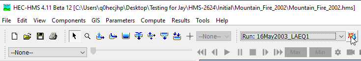
- Click on the Compute menu and select the Create Compute | Simulation Run option. A wizard window will open to guide you in creating a new simulation run. In the first step enter name 16May2003_LAEQ1.
Viewing Sediment Results
Within the HEC-HMS Results tab, both the clean water flow and sediment results can be viewed. The first half of the results under each element contains the typical clean water hydrologic outputs, such as excess precipitation, soil infiltration, and direct runoff (red box). When selecting Graph, Summary Table, and Time-Series Table immediately under the element, the results will only show the clean water outputs. The sediment computations are located in the Sediment folder. The Results tab provides sedigraphs for sediment load, sediment volume, and sediment concentration. The load and volume can be further broken down into their respective sediment type. 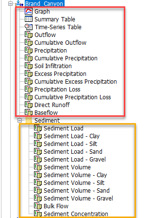
- Viewing Debris Yield Simulation Results.
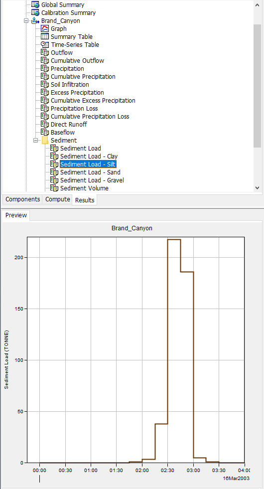
- Select the Result Tab and select the Sediment node under the Brand_Canyon subbasin element.
- Click through each sediment results to view the Sediment Load, Sediment Volume, and Sediment Concentration. These results represent the total value.
- Sediment results can broken out by sediment type. The image below shows the sediment load for the silt sediment type.
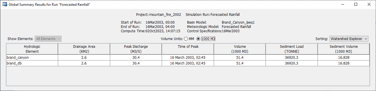
- Click on Global Summary to view the Global Summary Results table (the button is in the Result toolbar). The Global Summary Results table provides the clean water Peak Discharge value, clean water Time of Peak, clean water Volume, debris yield Sediment Load, and debris yield Sediment Volume.
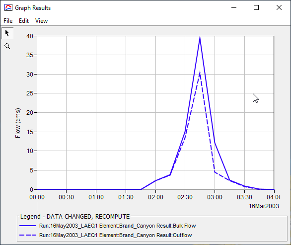
- Select the Bulk Flow result to view the combination of the clean water flow and sediment volume. This result combines the clean water Outflow with the total Sediment Volume (converted to a rate). The figure below was created by selecting the Bulk Flow and Outflow results (hold the Control key and select both results, then select the plot button in the results toolbar).
Question 3: Why is the value for the Clay Sediment Load zero?
Because clay was not included in the gradation curve. In the soil sample around the debris basin, there was no clay material.
Question 4: What is the estimated total sediment load with the forecasted rainfall amount on 16 Mar 2003?
36,920 TONNE
Question 5: What is assumed about the shape of the bulk flow hydrograph?
Assumes the peak of the sedigraph occurs at the same time as the flow hydrograph. The shape of the sedigraph can be changed by adjusting the Exponent parameter; however, the sedigraph and flow hydrograph peak value will always occur at the same time. This is generally not the case as the debris flow peak can happen relatively quickly following an intense rainfall/flow event.
Question 6: How confident do you feel about the results? What would be ways to improve your confidence?
Not confident. These results were computed from an initial guess at parameters. If there were measured volumes to compare, we can improve our confidence in the results. Otherwise, we can compare the results against other debris yield equations.
Set up Debris Yield methods for MSDPM, USGS EA, and USGS LT
- Parameterize the other debris yield methods, MSDPM, USGS-EA, and USGS-LT.
- Create 3 copies of the Brand_Canyon_LQEQ1 basin and rename the basins to include the debris yield method (i.e. Brand_Canyon_USGS-EA)
- Make sure in the Forecasted_Rainfall Meteorological Model to include Subbasins from the other basin models.
- Create 3 copies of the LA_EQ1 simulation and rename the simulation run to include the debris yield method. Make sure to select the correct Basin Model for each simulation.
- Run the simulations and review the results.

For MSDPM, set the Max 1-hr rainfall intensity and Total Min Rainfall Amount to zero for this test.
Question 7: Which method provides the best results?
The total Sediment Volume results are listed in the table below.
| Method | Volume (m^3) |
|---|---|
| LA EQ1 | 16,828 |
| MSDPM | 17,215 |
| USGS EA | 8,324 |
| USGS LT | 15,902 |
It is difficult to assess which method provides the best results without any measured volumes to compare; however, the LA EQ1, MSDPM, USGS EA, & USGS LT were derived from watersheds and debris basins within the Southern California mountain region. Without any adjustments to parameters, LA EQ1, MSDPM, USGS LT are relatively similar in total volume. USGS EA computes the smallest total volume. One consideration could be to average the estimates or take the median estimate. These methods are empirically derived with their own set of assumptions.