Download PDF
Download page Estimating Parameters with GIS Datasets.
Estimating Parameters with GIS Datasets
Last Modified: 2024-11-04 16:37:34.838
Software Version
HEC-HMS version 4.13 beta 3 was used to create this tutorial. You will need to use HEC-HMS version 4.13 beta 3, or newer, to open the project files.
Project Files
Continue using the project files from the previous Computing Subbasin and Reach Characteristics tutorial.
Overview
This tutorial will guide you through the steps of using the Expression Calculator in HEC-HMS to estimate initial transform and loss parameters. Transform parameters will be estimated using Subbasin Characteristics and loss parameters will be estimated using gridsets. The Expression Calculator can be launched from global editors.
For this tutorial, the gridded data has already been prepared for you. A separate tutorial demonstrates how to use the Grid Data Manager to import various GIS raster data for use in HEC-HMS.
Transform Parameter Estimation
All model and parameter components other than transform and loss parameters have been pre-configured for you.
- Open the Punx.hms project, if not already open.
- Select the Basin Model → Sep2018.

- The Transform method chosen for this model is ModClark. Open the Global Editor for ModClark by selecting Parameters→ Transform→ ModClark.

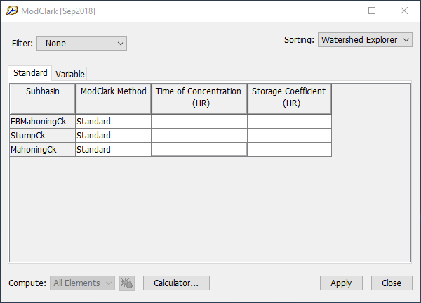
- The ModClark parameters are undefined; initial estimates need to be entered. The Expression Calculator is an easy way to quickly populate initial parameter estimates for each subbasin. Select the Calculator... button (shown below) to launch it.


- The Expression Calculator can access two types of data: Grids (external grids that have been imported into HEC-HMS via the Grid Data Manager) and Stats (the computed Basin Characteristics values). We will use the Stats tab to compute initial estimates for Time of Concentration. In the Expression Calculator, ensure that the Field: Time of Concentration is selected and then select the Stats tab to access the Basin Characteristics variables.

- For this tutorial, we are going to use the equation below, which was developed for the modeling area of interest, to estimate Time of Concentration. This equation establishes a relationship between Longest Flowpath Length (L) in miles, Centroidal Flowpath Length (LC) in miles, and 10-85 Slope in feet per mile. It is important to note that these types of equations are usually developed for use within specific watersheds and are not always applicable to other regions, land cover types, soil types, etc. Care should be taken in choosing/developing an equation that applies to the modeling area of interest. For simplicity, we will assume an R/(TC+R) relationship of 0.5 which means that the Storage Coefficient (R) will be equal to the Time of Concentration (TC).
- T_c = 2.2 * \frac{(L*L_C)}{\sqrt{Slope_{10-85}}}^{0.3}
- \frac{R}{T_c+R}= 0.5
In the Time of Concentration equation box, you can enter the above TC equation by double-clicking variables, functions, and entering numbers as appropriate. For simplicity, click the Copy button in the CODE text box below (located in the upper right corner) and then paste it into the Time of Concentration equation box in HEC-HMS. Select Calculate when finished. Notice how the global editor automatically populates with Time of Concentration estimates.
2.2 * (pow(([Longest Flowpath Length (MI)] * [Centroidal Flowpath Length (MI)]) / (pow([10-85 Flowpath Slope (FT/MI)],0.5)),0.3))CODE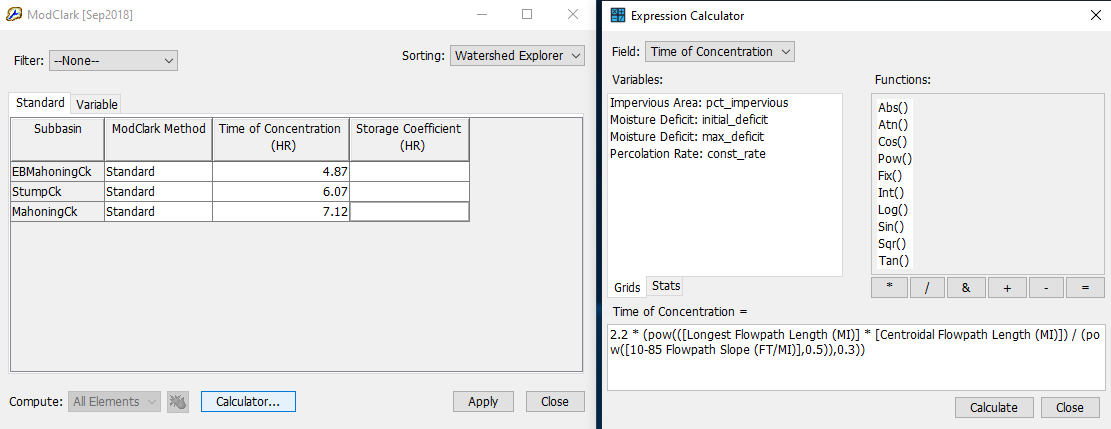
- Since we are assuming an R/(TC+R) relationship of 0.5, the initial Storage Coefficient estimate will equal the Time of Concentration calculation. Within the Expression Calculator window, select Field: Storage Coefficient, then, using the same equation as before, select Calculate, and then select Close. Within the ModClark Global Editor window, select Apply to save the initial estimates and then select Close.
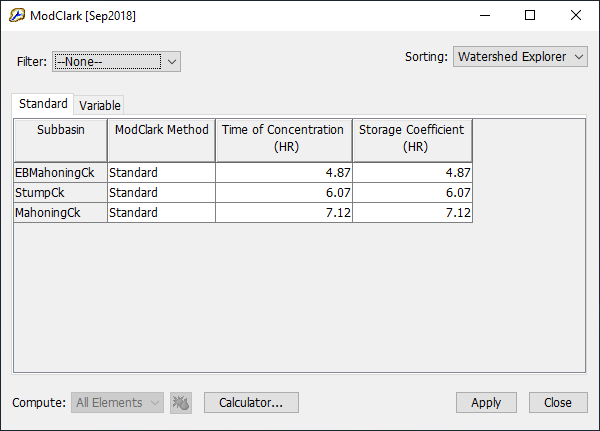
- Notice how the Expression Calculator populates the global editor with three significant digits. This can be changed by selecting Tools→ Program Settings→ Compute and then adjusting the Expression calculator precision toggle box. For this tutorial, you can leave the precision to the default value of 3.
- Select the Basin Model → Sep2018.
Loss Parameter Estimation
- Following the same general workflow, we can establish loss parameter estimates using gridded data.
- The Loss method chosen for this model is Deficit and Constant. Open the Global Editor for Deficit and Constant by selecting Parameters→ Loss→ Deficit and Constant.

- The Loss parameters are undefined; initial estimates need to be entered. Select Calculator... to launch the Expression Calculator.

- Make sure to set the Field: to Initial Deficit and make sure that the Grids tab is selected.

- Notice how four different variables are available in the Expression Calculator. This is because four different loss grids have already been imported for your use via the Grid Data Manager and can be accessed by the Expression Calculator. More info on Grid Data can be found in the HEC-HMS Manual.
- Double-click Moisture Deficit: initial_deficit to enter the variable into the Initial Deficit equation box and select Calculate. Notice how the global editor automatically populates with Initial Deficit estimates. Repeat this step by selecting the three other variables in the Expression Calculator to estimate Maximum Storage, Constant Rate, and Percent Impervious. When finished, select Close in the Expression Calculator window. Within the Deficit and Constant Global Editor window, select Apply to save the initial estimates and then select Close.

- The Loss method chosen for this model is Deficit and Constant. Open the Global Editor for Deficit and Constant by selecting Parameters→ Loss→ Deficit and Constant.
Results
- Now that the Transform and Loss parameters have been estimated with Basin Characteristics data and Grid data, you can make a simulation run and view the results. A Sep2018 run has already been setup for you.
- Start a simulation by selecting the Compute tab, then right-click on Sep2018, and select Compute.

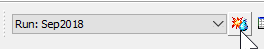
- Alternatively, you can also select the Sep2018 simulation on the toolbar and click on the compute raindrop button.
- Start a simulation by selecting the Compute tab, then right-click on Sep2018, and select Compute.
- Once the compute is complete, close the compute progress bar and navigate to the Results tab. Under the Simulation Runs folder, review your results by expanding the Sep2018 simulation and clicking through your model elements. When you are done reviewing your results, click on the Outlet element and select Graph. The graph below in question 1 should appear showing the combined simulated flow (blue lines) compared with the observed flow (black dotted lines).
Question
- How do the computed results compare to the observed data at the outlet?

There are some common trends between the computed and observed data, but improvements should definitely be made to the initial parameter estimates. The takeaway from this tutorial is that the Expression Calculator can assist in quickly populating the global editors with initial estimates or guesses, but there is no substitute for calibration when observed data is available. Model calibration will be covered in a separate tutorial.

This tutorial concludes the Applying HEC-HMS GIS Parameter Estimation Tools tutorial group.