Applying the Interpolated Precipitation Grid Option within the Truckee River Watershed - No Bias Option

HEC-HMS version 4.10 beta 5 was used for this example. 

Introduction

Utilizing gridded data in an HEC-HMS model is beneficial because gridded products can better capture the temporal and spatial variability of meteorologic data across a watershed when compared to gage measurements at a single point. However, hourly or sub-hourly gridded products, such as Multi-Radar Multi-Sensor (MRMS) Quantitative Precipitation Estimate (QPE), Snow Data Assimilation System (SNODAS), or Next Generation Radar (NEXRAD), are not always available, particularly for historic events of interest to the modeler. In these cases, a gridded dataset can be created by interpolating point observations of climatological variables recorded at weather stations.

In HMS version 4.10 and above, interpolated grids can be developed for shortwave radiation, precipitation, temperature, windspeed, dew point temperature, and evapotranspiration. This tutorial demonstrates how gaged precipitation measurements can be interpolated to create a gridded precipitation dataset using an existing model of the Truckee River basin in the western United States. The Truckee River basin is in the Sierra Nevada mountains and straddles the border of California and Nevada.

Download the initial HEC-HMS project files here - Truckee_River_Initial.zip

Inspect Precipitation Data

Navigate to the data subfolder in the Truckee River model directory and open the Jan_1997_gage_precipitation.dss file in HEC-DSSVue. Inspect the precipitation timeseries in the DSS file. The E-part of the timeseries entry shows that all of the gage data has an hourly timestep. The C-part of each timeseries is named PRECIP-INC. Note the C-part must be named PRECIP-INC for HEC-HMS to read the gaged precipitation data. A C-part of PRECIP-INC indicates the data is incremental and has the PER-CUM data type. The PER-CUM data type is for data representing the cumulative depth of precipitation that occurred in each time interval. Tabulating the data, as shown below, reveals the units (INCHES) and data type (PER-CUM) are consistent for each time-series. It is important all precipitation timeseries used in the HMS model have consistent units and data type. You can use DSSVue to edit the C-part pathname, units, and data type if needed. 

Data can be converted to the PER-CUM data type in HEC-DSSVue by using Math Functions | Time Functions | Min/Max/Avg/… Over Period | Accumulation over Period and setting the New Period Interval accordingly (e.g., 1HOUR).

Now, open the Truckee River HEC-HMS model and navigate to the Time Series Data folder in the Watershed Explorer. View the precipitation gages contained in the model, as shown below. Note the DSS filename for each gage is set to the Jan_1997_gage_precipitation.dss file, and the DSS pathname is properly referenced. Also note the latitude and longitude of each gage has been entered. If the latitude and longitude is not specified, the gage cannot be used for interpolation. The tree for each precipitation gage can be expanded further to show the Time Window, Table, and Graph tabs. However, these tabs are not necessary if the gage data source references a DSS file.

The figure below shows the location of all the precipitation gages in the model relative to the Truckee River watershed. A shapefile of the precipitation gages is included in the maps subfolder in the model directory. Note the limited number of precipitation gages within the watershed and the drastic differences in elevation across the basin. The lowest elevation in the watershed is 4,450 feet, and the highest elevation is 10,300 feet.

Create an Interpolated Precipitation Grid

Unlike other gridded data tools in HEC-HMS, (like the Normalizer and Importer tools) the setup and specifications for gage interpolation are entirely contained within the meteorological model interface. The actual interpolation computation is conducted when a simulation using the meteorological model is computed. The interpolated grid files are written to the meteorological model's DSS file.

Configure the Meteorological Model

The Jan_1997_gageInterp meteorological model is already included in the Truckee River HEC-HMS project. Select this meteorological model and inspect the Component Editor. Currently, the Precipitation method is set to None. Change the Precipitation method to Interpolated Precipitation, as shown below. 

Expand the meteorological model tree and select Interpolated Precipitation node to open the Component Editor, as shown below.

In the Interpolated Precipitation Component Editor, set the interpolation method to Inverse Distance. The inverse distance interpolation method assumes the weight, or influence, of a gage is equal to the inverse of its distance from the interpolated cell, which is a good assumption for precipitation data. Other interpolation methods, including Inverse Distance Squared, Nearest Neighbor, and Bilinear, are also available and may be more applicable when interpolating grids for other climatological variables. For this tutorial, keep the adjustment method set to None. In the Gage table, select each precipitation gage in the model, and assign it a radius of influence of 31 miles (50 kilometers). The radius of influence, shown for each gage on the map in the figure below, is the maximum distance that the gage will be included in the interpolation. Beyond its radius of influence, the gage will not affect the cell values of the interpolated grid. 

If a gage included in the interpolation does not have any data for a given timestep, that gage will be excluded from the interpolation for that timestep.

The figure below shows the Interpolated Precipitation dialog box after all gages have been added.

Compute the Interpolated Grids

To compute the interpolated grids, a simulation must be computed that uses the meteorological model. The Jan_1997_precipInterp simulation run already included in the Truckee River HEC-HMS model is set up to use the Jan_1997_gageInterp meteorological model. To run the simulation, navigate to the Compute tab, right-click on the Jan_1997_precipInterp simulation, and select the Compute button.

Spatial results were turned on for this simulation. Within the Spatial Results toolbar, select the Cumulative Precipitation results, as shown below. Note, the terrain has been deselected in the Map Layers so the spatial results are easier to see. You can right click within the spatial results map to see a menu option to plot a time-series of the cumulative precipitation for each grid cell in the basin model. You can also visualize temperature and other simulated results. 

After the compute is complete, navigate to the Jan_1997_gageInterp.dss file in the HEC-HMS model directory, as shown below. This is the DSS file associated with the Jan_1997_gageInterp meteorological model. 

Open the DSS file and filter to only include data with the C-part PRECIPITATION, as shown below. All of the filtered files shown are the interpolated precipitation grid files.

View Simulation Results

Navigate to the Results tab of the Watershed Explorer and select the Jan_1997_precipInterp simulation. To view the simulation results at a junction or other model element, select the model element in the tree and select Graph, as shown below.

View the simulation results at the SouthLakeTahoe, MartisCreek_IN, Reno, and Steamboat junctions, as shown below.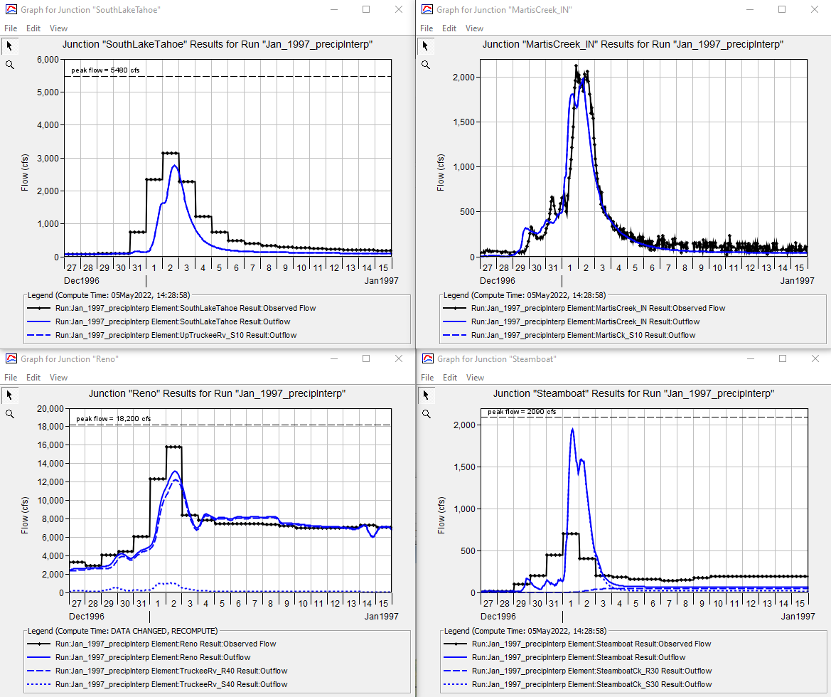

The simulation results appear to reasonably capture the timing of runoff throughout the watershed. However, the model consistently underestimates peak discharge. This could be due to a number of factors, such as the lack of a dense gage network within the watershed, the calibration parameters adopted for the model, or inaccurate gage measurements. Generally, gaged precipitation measurements are considered higher quality than radar or modeled precipitation estimates, so the gage measurements likely characterize the precipitation that fell at the gage location very well. However, in mountainous regions like the Truckee River watershed, most weather stations are located in populated areas at relatively low elevations. Since more precipitation generally occurs at higher elevations, a precipitation grid interpolated from data at low-lying weather stations is likely to underestimate precipitation in higher areas of the watershed. To account for differences in elevation when interpolating gaged precipitation measurements, HEC-HMS allows the user to bias the interpolated grids using another gridded dataset, such as PRISM, that more accurately accounts for differences in elevation in gridded precipitation estimates. For a tutorial showing how to use the Bias adjustment method, see Applying the Bias Option when Interpolating Precipitation within the Truckee River Watershed.

Download the final HEC-HMS project files here - Truckee_River_Final.zip

Other Useful Links

NCEI Hourly/Sub-Hourly Observational Data
National Weather Service Cooperative Observer Program (COOP) Data Download
PRISM Climate Group