Applying the Bias Option when Interpolating Precipitation within the Truckee River Watershed

HEC-HMS version 4.10 beta 5 was used for this example. 

Introduction

Creating a gridded precipitation dataset by interpolating gage measurements can more accurately capture the distribution of rainfall across a watershed than simply applying uniform rainfall amounts to each subbasin. However, it is important to consider how the location of each gaging station will influence the interpolated grid values. In many cases, particularly in mountainous regions where elevation, aspect, and other factors play a major role in the magnitude of precipitation, interpolated grid values could be biased. If, for example, the gaging stations are located at lower elevations, as is often the case, the interpolated grid cells will likely underestimate the magnitude of precipitation in areas of the watershed where the elevation is much higher.

In HMS 4.10 and above, interpolated precipitation grids can be adjusted using a bias grid. See Bias Adjustment Method Computation for a demonstration of how the bias adjustment computation works. The bias grid is a gridded dataset that captures the normal, or expected, spatial distribution of precipitation over the watershed. One type of grid that can be used to bias an interpolated precipitation grid is a 30-year normal or monthly precipitation grid from the Parameter-elevation Relationships on Independent Slopes Model (PRISM). Since PRISM accounts for differences in elevation across the landscape when estimating precipitation, using PRISM data to adjust interpolated precipitation grids can often lead to a better estimate of rainfall across a watershed. This tutorial demonstrates how to use a bias grid to adjust an interpolated precipitation grid using an existing HMS model of the Truckee River basin in the western United States. The Truckee River basin is in the Sierra Nevada mountains and straddles the border of California and Nevada.

Download initial project files here - Truckee_River_Initial.zip

Inspect Existing Model

Open the Truckee River model and view the Jan_1997_gageInterp meteorological model. Notice the model has both a rainfall and a snowmelt component. This tutorial focuses on the rainfall component. Expand the tree and select Interpolated Precipitation. The precipitation grid has been interpolated from data at 26 weather stations, each with a radius of influence of 31 miles (50 kilometers). The location and elevation of each weather station in the model is shown below.

Note the maximum elevation of the Truckee River watershed is nearly 10,300 feet. However, none of the weather stations are above 7,000 feet, and only a handful are above 5,000 feet. Since the magnitude of rainfall generally increases with elevation, the precipitation grid interpolated from these weather stations likely underestimates the magnitude of precipitation that fell at higher elevations in the basin.
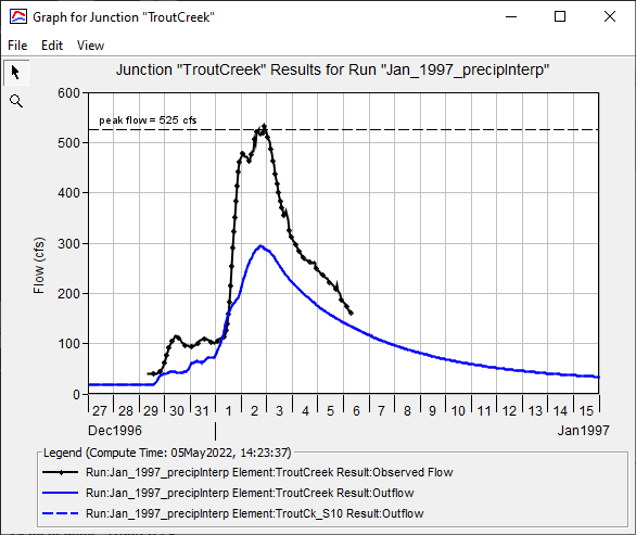
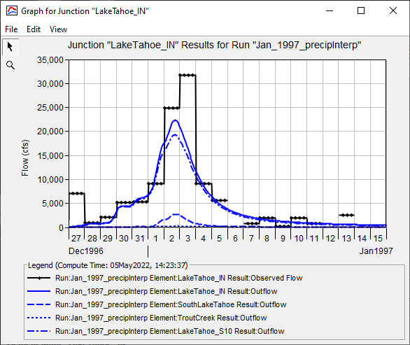
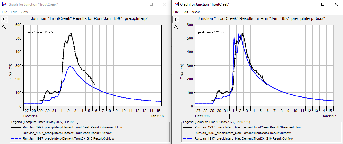
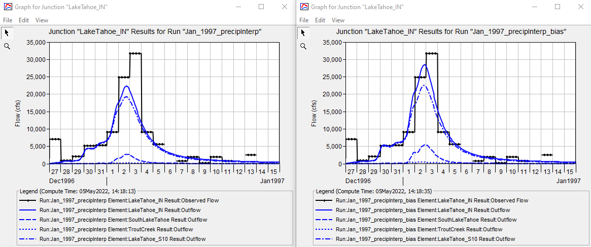
To verify the interpolated precipitation grid underestimates precipitation at high elevations in the watershed, navigate to the Results tab of the model and expand the Jan_1997_precipInterp simulation run. Graph the results at the SouthLakeTahoe, TroutCreek, and LakeTahoe_IN junctions. As shown in below, the simulated runoff is much lower than what was observed at these locations.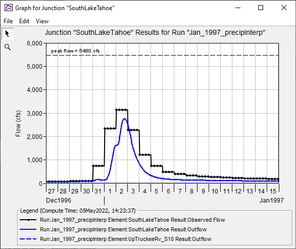

Create a New Meteorological Model

To adjust the interpolated precipitation grids using the bias adjustment method, first create a new meteorological model by navigating to the Components tab of the model, right-clicking on the Jan_1997_gageInterp meteorological model, and selecting Create Copy, as shown below.

Name the new meteorological model Jan_1997_gageInterp_bias. Then, select the Interpolated Precipitation component of the new meteorological model. In the Interpolated Precipitation dialog box, change the Adjustment Method from None to Bias. In the Grid Name dropdown, select the PRISM_Precipitation_Normals grid, as shown below.

Examine the PRISM_Precipitation_Normals Grid File

The PRISM_Precipitation_Normals grid is a 30-year normal precipitation grid for the United States. See Importing and Using Parameter-elevation Regressions on Independent Slopes Model (PRISM) Precipitation Data for a tutorial describing how to download and import PRISM data into HEC-HMS. The grid data has been previously added to the model as a Precipitation-Normal Grid. It is important to note that a grid cannot be used as a bias grid for interpolated precipitation unless it is added to the model as a Precipitation-Normal Grid. To view the PRISM_Precipitation_Normals grid data, navigate to the Grid Data component of the model and expand the Precipitation-Normal Grids tree, as shown below.

Precipitation Bias Grids

There are many options for precipitation bias grids. Ideally, you would use total storm grids for the specific event being modeled. For example, the daily PRISM dataset could be cumulated for the storm event in this example. Another option is the 1% annual chance exceedance precipitation frequency grid from NOAA Atlas 14.

Select the PRISM_Precipitation_Normals grid and select the icon next to the DSS Pathname to open the DSS file where the grid data is located, as shown below.

In the DSS file that appears there is a single grid spanning the period 31 Dec 1980 to 31 Dec 2010. Each grid cell is equal to the average, modeled precipitation at that grid cell over the 1980-2010 period. Note there is only one grid in the DSS file, and only a single grid record can be selected as the bias grid. This is because only one grid is used to adjust the interpolated precipitation values. While interpolated grids are computed for hourly or daily timesteps, the same bias grid is used for each computation. Because only a single bias grid is used for all timesteps, the bias grid should take into account long-term averages or cumulative totals, like the 30-year normals used in this tutorial or monthly totals. Right-click on the grid file and select Plot. It is clear the PRISM grid covers the entire continental United States, as shown below. This is important, as the bias grid must cover all precipitation gages used to develop the interpolated precipitation grid. The bias grid does not need to have a specific projection or cell size, as it will be reprojected to the discretization projection of the HMS model prior to performing any interpolation computations.

If the extent of the normal grid is not clear from plotting the grid in the DSS viewer, additional information about the grid extents can be found by selecting the Grid Info tab above the plot, as shown below.

Compute the Bias-Adjusted Grids

To compute the bias-adjusted, interpolated grids, a simulation run must be computed that uses the new meteorological model. To create a new simulation, select the Compute | Create Compute | Simulation Run, as shown below.

Name the new simulation Jan_1997_gageInterp_bias. Select the Jan_1997 basin model, the Jan_1997_gageInterp_bias meteorological model, and the Jan1997 control specifications. Then select Finish. Open the Component Editor for the new simulation run and turn on Spatial Results at a 1 Hour time step. Right-click on the new simulation run and select Compute, as shown below.

Compare Simulation Results

To view the effect of the bias adjustment on the interpolated grids, navigate to the Results tab and expand the Jan_1997_precipInterp_bias simulation run. Graph the SouthLakeTahoe, TroutCreek, and LakeTahoe_IN junctions. As shown in the figures below, simulated runoff is higher when using the bias-adjusted grids than when using the unadjusted grids.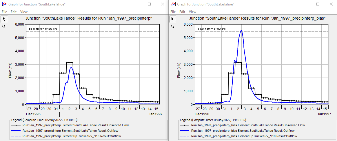

The following images show the cumulative precipitation displayed using spatial results. Notice that the gage only interpolation results show minimum/maximum precipitation values at cells co-located with precipitation gages. When using a bias grid, the minimum/maximum precipitation values are correlated with the spatial pattern contained in the bias grid (more precipitation at higher elevations). 

Conclusion

The bias-adjusted precipitation interpolation simulation did result in improved model results. Some of the error in the simulated results could be due to the temperature grids used for the snowmelt component. Model parameters could probably be adjusted to better match the observed peaks, but it is possible the magnitude of precipitation in the interpolated grids is simply too low, even after the bias adjustment. This could be due to a number of factors, the most important of which is the distribution of weather stations throughout the watershed, or the selected bias grid (a storm total bias grid might provide better results). As shown in the figures above, there are only three precipitation gages in the Truckee River basin. There are others just outside the basin, but the variability of precipitation in mountainous regions is well-documented. Due to orographic effects, a large amount of precipitation can fall on one side of a mountain while very little falls on the other side. Because of this, gage measurements at a nearby weather station may not be representative of precipitation totals several miles away. Bias-adjusting the interpolated precipitation grids helps to account for differences in elevation and improve gridded precipitation estimates, but the quality and distribution of observed gage measurements still has the greatest impact on the accuracy of the final, interpolated grids.

Download final project files here - Truckee_River_Final.zip

Other Useful Links

NCEI Hourly/Sub-Hourly Observational Data
National Weather Service Cooperative Observer Program (COOP) Data Download
PRISM Climate Group