Calibrate the Basin Model to Historical Data using Daily Precipitation and Temperature Dataset

This tutorial was not designed to provide guidance for applying downscaled climate model projections to inform an analysis. Each Federal, State, and Local agency should follow agency specific guidance for including possible future climate change information in hydrologic analysis. This tutorial highlights tools in HEC-HMS that aid modelers in making use of gridded meteorologic datasets and utilizing the new Ensemble compute option to organize many simulations. 

An existing HEC-HMS model of the Success Dam watershed was used for this example. The existing model had been calibrated using hourly precipitation and temperature boundary conditions along with hourly streamflow observations. As mentioned, the model was re-calibrated because the CMIP5 Climate Projection datasets are available at daily time scales. Precipitation intensities and temperature measurements that can be captured with hourly observations are not available when using daily accumulated or average data for boundary conditions. When you look at the example HEC-HMS model, the simulation used for calibration was named POR_Calibration. The simulation time window was from 01 October 1970 through December 31, 2005. 

The model performance was evaluated using Snow Water Equivalent (SWE), monthly average streamflow, and annual maximum peak flow information. Daily average "observed" flow was available for the reservoir (computed inflow into the reservoir). The Success_Inflow discharge gage was added to the HEC-HMS model. Observed inflow is available for water years 1973 through 2005. The University of Arizona SWE dataset (https://nsidc.org/data/nsidc-0719/versions/1#anchor-2) was used as “observed” SWE within the example project. The gridded SWE data for water years 1982 - 2005 was downloaded from https://climate.arizona.edu/data/UA_SWE/. The University of Arizona SWE dataset was processed using the HEC-HMS Gridded Data Importer and Grid to Point tools. The HEC-HMS Grid to Point tool was only used to process the gridded University of Arizona SWE dataset for the MF_TuleR_S20 subbasin. The subbasin average University of Arizona SWE time-series was added to the HEC-HMS as an "observed" SWE gage (named SFTuleR_S20_UofA) and linked to the MF_TuleR_S20 subbasin element.  

Reference for University of Arizona SWE Dataset

Broxton, P., X. Zeng, and N. Dawson. (2019). Daily 4 km Gridded SWE and Snow Depth from Assimilated In-Situ and Modeled Data over the Conterminous US, Version 1 [Data Set]. Boulder, Colorado USA. NASA National Snow and Ice Data Center Distributed Active Archive Center. https://doi.org/10.5067/0GGPB220EX6A. Date Accessed 08-25-2022.

The following steps describe the process to calibrate the Tule River basin model.

1. A Control Specifications (named POR_Calibration) was added to the project for the period 01 October 1970 through 30 September 2005 using a simulation time-step of 3 hours. The HEC-HMS model was run at a 3-hour time step. The time step was increased to three hours because the meteorologic data was at a daily time step (running at smaller time steps does not really provide a benefit). The time step was not increased to 1-day because this would have introduced numerical diffusion issues in the transform calculations.
2. A Simulation Run (named POR_Calibration) was added to the project. The simulation combined the TuleRiver_Caibrated Basin Model, Livneh Meteorologic Model, and POR_Calibration Control Specifications. It took HEC-HMS approximately 2 minutes to run the 35-year time window. Approximately 20 iterations were needed to manually adjust parameter values to calibrate the model.

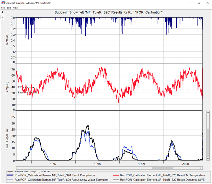
3. First, the temperature index model parameters were adjusted to calibrate the models performance in simulating SWE. The PX and Base temperature parameters were adjusted to improve the model's performance in matching the annual maximum SWE. The Dry Melt function was adjusted to improve the model's performance in matching the late season snowmelt pattern. The figure below shows the Snowmelt plot for the MF_TuleR_S20 subbasin element. For the four years shown, the HEC-HMS model does a good job matching the University of Arizona SWE. 
   
   The following figure shows the summary table from the POR_Calibration simulation. The Nash-Sutcliffe efficiency score was 0.83 for the period 1982 – 2005.
   
   The following table and plot show the simulated and University of Arizona monthly average SWE. The HEC-HMS model is able to reproduce the monthly trend and magnitude of SWE.

   MF_TuleR_S20 Monthly Average SWE (in)
   	HEC-HMS	University of Arizona
   January	7.7	6.4
   February	9.2	9.1
   March	8.2	9.8
   April	6.0	6.9
   May	2.8	3.1
   June	0.5	0.8
   July	0.0	0.0
   August	0.0	0.0
   September	0.0	0.0
   October	0.0	0.1
   November	1.0	0.7
   December	3.9	3.2
   Average Annual SWE	3.27	3.34

   
   

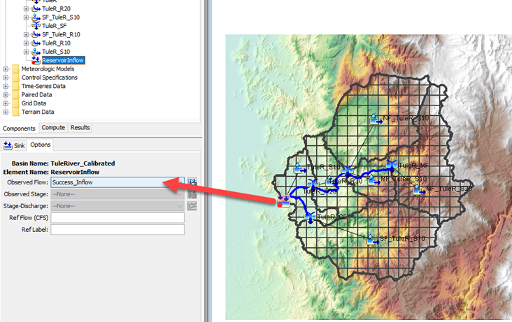
4. As shown below, the observed discharge gage Success_Inflow, was added to the sink element named ReservoirInflow.  
   
5. The subbasin elements in the basin model were configured to use methods appropriate for continuous simulation.
   1. The Simple Canopy method was selected, which is required for the model to simulate soil moisture conditions. Because daily precipitation and temperature data was used to drive the simulations, the option to compute evapotranspiration during both wet and dry time steps was selected (otherwise evapotranspiration would only be computed during time steps with no precipitation or snow melt).
   2. The Deficit and Constant loss method was selected. The Deficit and Constant method simulates the moisture state of the soil layer and infiltration into the soil. The maximum deficit parameter represents the total amount of storage in the soil (between field capacity and wilting point). You can estimate this parameter by determining how much precipitation is needed to generate runoff when the watershed has not received precipitation for an extended period. This parameter is easily estimated in continuous simulation by evaluating the model’s performance and looking for flow events after prolonged dry periods. The constant loss rate represent infiltration into the soil after the soil has reached field capacity.
   3. The ModClark transform method was selected. The ModClark parameters were finalized in the initial model calibration effort and not adjusted when using the Livneh and CMIP5 Climate Projection datasets.
   4. The Linear Reservoir baseflow method was selected. This method accepts infiltration from the Deficit and Constant method (only when there is no moisture deficit). Three linear reservoir baseflow layers were selected. The first layer was used to model interflow processes, the second layer was used to model slower responding baseflow processes, and the third layer was used to model the slowest responding groundwater return flow.
6. When calibrating the model, the Maximum Deficit, Constant Loss Rate, and Linear Reservoir Baseflow parameter were adjusted.
   1. The Maximum Deficit parameter was adjusted to improve the model’s performance in simulating runoff as the watershed transitioned from dry conditions in the summer to wet conditions in the fall/winter.
   2. The Constant Loss Rate was adjusted to improve the model's performance in matching peak flows.
   3. The Linear Reservoir baseflow method parameters (fraction, coefficient, and number of linear reservoirs in series) were adjusted to improve the model's performance in simulating the hydrograph shape and baseflow recession. The fraction parameter was impactful in matching observed runoff volume. The coefficient and number of linear reservoirs in series parameters were impactful in matching the monthly flow distribution.
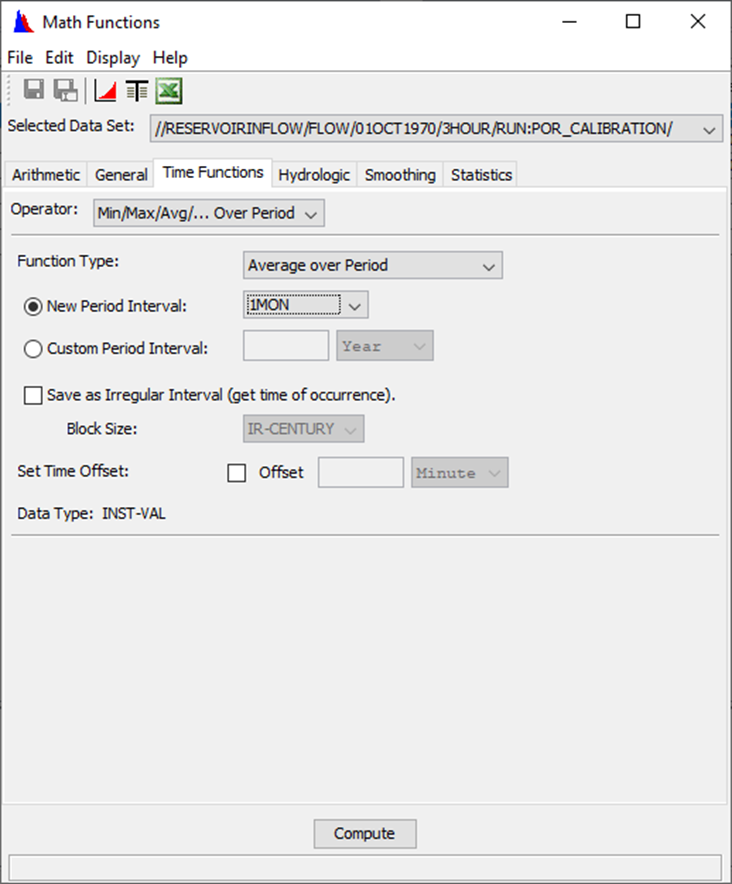
7. HEC-DSSVue was used to convert the HEC-HMS model results from 3-hour (SWE and flow) to daily and monthly values. The daily average observed flow at Success Dam (ReservoirInflow element) was also converted to monthly average flow. The figure below shows the HEC-DSSVue Time Functions tab. The Average over Period option was selected. In the figure, a period of a Month was selected.
   

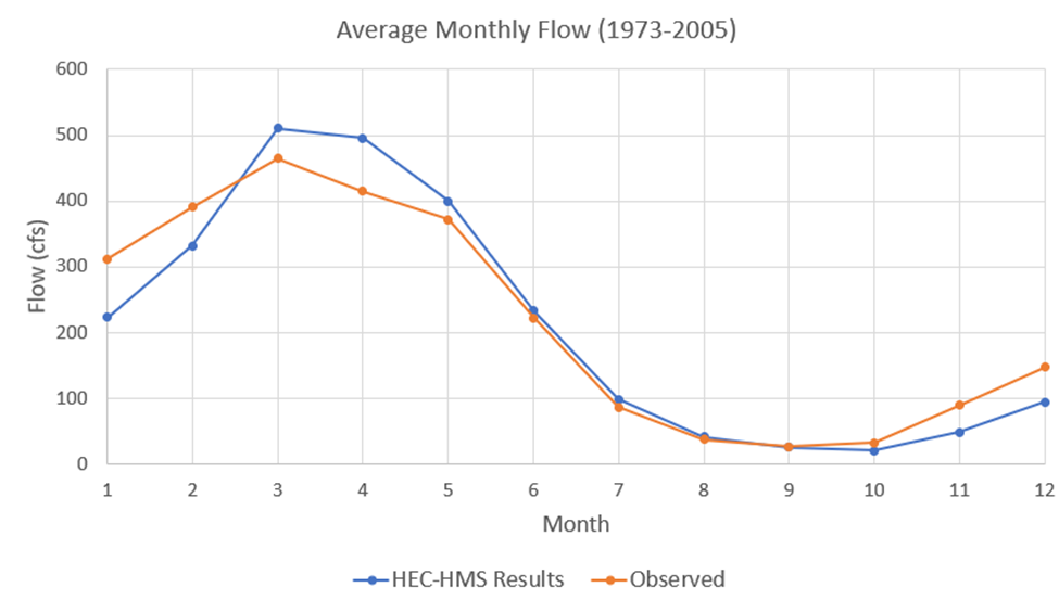
8. The model’s performance was evaluated by comparing monthly average flow and annual peak flows. The table and figure below show the average monthly flows for the period (1973 - 2005). When evaluating simulated and monthly average flows, the Nash-Sutcliffe efficiency score was 0.7 and the Percent Bias in flow was -2.63 percent. The HEC-HMS model is able to reproduce the monthly flow response in the Tule River watershed (the monthly average flow results also reflect good performance in snow accumulation and melt as snowmelt drives the runoff pattern in the spring months).

   ReservoirInflow Monthly Average Flow (cfs)
   	HEC-HMS	Observed
   January	223	312
   February	331	391
   March	510	465
   April	496	415
   May	400	371
   June	233	222
   July	98	86
   August	41	37
   September	25	26
   October	21	32
   November	48	89
   December	94	147
   Average Annual Flow	210	216

   

9. The model was also evaluated at how well it was able to reproduce the flow frequency response for the watershed upstream of Success Dam. HEC-SSP was used to compute the daily average flow frequency curve for the observed and computed inflow into Success Dam. The daily averaged observed and HEC-HMS model results were imported into an HEC-SSP project using the Data Importer. Then, annual maximum peak 1-day average flows were extracted from the time-series using a Filter Data option in HEC-SSP.  
   Separate Bulletin 17 Analyses were created for the observed data and HEC-HMS peak 1-day average flows. The flow frequency analysis was performed for water years 1973 - 2005 (33 years). The figures below show results from the flow frequency analyses. The HEC-HMS model results generated a similar 1-day flow frequency curve for inflow into Success Dam as the observed dataset, especially for higher flows.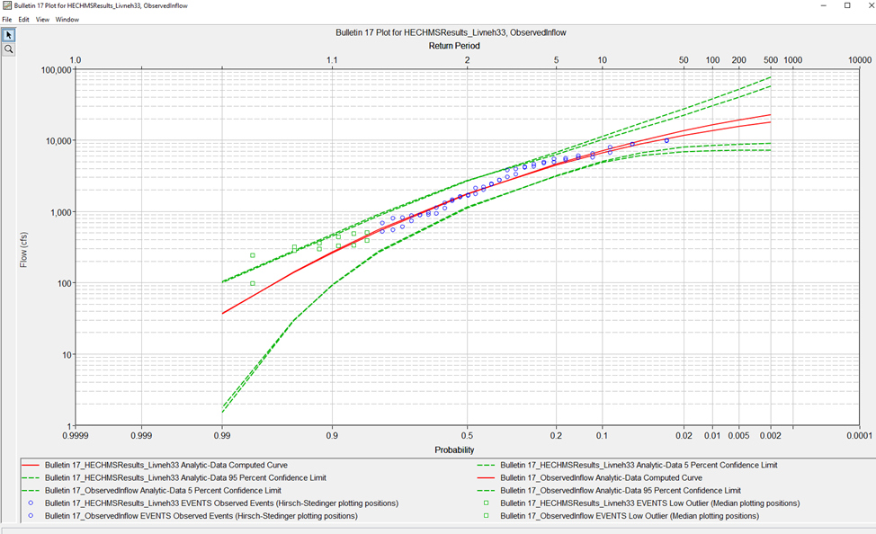
   

At this point the HEC-HMS model was considered calibrated and ready for application of the CMIP5 Climate Projection datasets. As mentioned, approximately 20 iterations of parameter adjustment, model simulation, and results evaluation went into the model calibration effort. Additional work could have gone into calibration; however the calibration effort was stopped once model performance was adequate. The calibration effort took 2 hours to complete. 

Continue to Create Ensemble Analysis Simulations for Downscaled Climate Model Datasets.