Download PDF
Download page Creating an Ensemble Analysis Compute.
Creating an Ensemble Analysis Compute
Last Modified: 2022-10-03 12:54:35.441
This tutorial demonstrates the new Ensemble Analysis compute option in HEC-HMS.
Software Version
HEC-HMS version 4.11 beta 3 was used to create this example. You can open the example project with HEC-HMS 4.11 beta 3 or a newer version.Introduction
Ensemble modeling is a process whereby multiple base models are created and simulated in a collective fashion to predict an outcome. Each base model may include different basin configurations, modeling methods, parameter sets, initial conditions, and/or boundary conditions. As long as the base models are diverse and independent, the prediction error of the base models decrease when the ensemble modeling approach is used. While the ensemble model is composed of multiple models, it acts and performs as a single model.
In this tutorial and guide, each base model was assigned a different precipitation data source to model the same, continuous event. The corresponding basin model was then calibrated based on the precipitation data source that was applied to it. In hydrologic modeling, the boundary conditions assigned to a model are often a significant source of uncertainty. An ensemble analysis can be created to aggregate the prediction of each base model and to reduce the uncertainty in the modelled predictions.
Description of Watershed
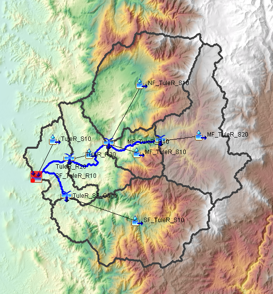
Success Dam (now commonly known as Schafer Dam) is located on the Tule River just upstream of the town of Porterville, California. The HEC-HMS project in this example includes Success Dam as the most downstream basin element and an upstream catchment area of approximately 390 square miles.
Description of Meteorological Data Sources
This HEC-HMS project consists of six different meteorologic models, each of which uses a different precipitation data source to model a continuous event spanning the entire months of January and February, 2017. These data sources include Analysis of Period of Record for Calibration (AORC), Interpolated Gages, Interpolated Gages with Bias Grid, Multi-Radar Multi-Sensor (MRMS), AORC data normalized to Parameter-elevation Regressions on Independent Slopes Model (PRISM) volumes, and MRMS data normalized to PRISM volumes. Details of some of these data sources, along with other commonly used sources of gridded hydrologic data, can be found here. A separate tutorial and guide titled Correcting Precipitation Volume with the Normalizer Utility details how to use PRISM data in conjunction with other precipitation datasets to correct the volume estimates.
Description of the Basin Model and Simulation Runs
The six basin models used in this HEC-HMS project each use the same methods (simple canopy, deficit and constant loss, modified Clark transform, linear reservoir baseflow, and gridded temperature index snowmelt). Six simulation runs were created, each with a basin model, a corresponding meteorologic model, and a control spec assigned to it. Each of the basin models have different calibrated parameter values due to the different precipitation data sources applied to them. Below are tables that show the calibrated loss, transform, and baseflow parameter sets from each of the six basin models.
| Deficit and Constant Loss Rate Parameters | |||||
|---|---|---|---|---|---|
| Basin Model | Subbasin | Initial Deficit (IN) | Maximum Storage (IN) | Constant Rate (IN/HR) | Impervious (%) |
TuleRiver_AORC | MF_TuleR_S20 | 0.7 | 8 | 0.2 | 0.0 |
| NF_TuleR_S10 | 0.7 | 8 | 0.2 | 0.0 | |
| MF_TuleR_S10 | 0.7 | 8 | 0.2 | 0.0 | |
| TuleR_S20 | 0.7 | 8 | 0.2 | 0.0 | |
| SF_TuleR_S10 | 0.7 | 8 | 0.15 | 0.0 | |
| TuleR_S10 | 0.7 | 8 | 0.2 | 0.0 | |
TuleRiver_Interpolated | MF_TuleR_S20 | 1 | 8 | 0.4 | 0.0 |
| NF_TuleR_S10 | 1 | 8 | 0.4 | 0.0 | |
| MF_TuleR_S10 | 1 | 8 | 0.2 | 0.0 | |
| TuleR_S20 | 1 | 8 | 0.2 | 0.0 | |
| SF_TuleR_S10 | 1 | 8 | 0.25 | 0.0 | |
| TuleR_S10 | 1 | 8 | 0.2 | 0.0 | |
TuleRiver_InterpolatedBias | MF_TuleR_S20 | 1 | 8 | 0.4 | 0.0 |
| NF_TuleR_S10 | 1 | 8 | 0.4 | 0.0 | |
| MF_TuleR_S10 | 1 | 8 | 0.4 | 0.0 | |
| TuleR_S20 | 1 | 8 | 0.4 | 0.0 | |
| SF_TuleR_S10 | 1 | 8 | 0.4 | 0.0 | |
| TuleR_S10 | 1 | 8 | 0.4 | 0.0 | |
TuleRiver_MRMS | MF_TuleR_S20 | 1 | 8 | 0.28 | 0.0 |
| NF_TuleR_S10 | 1 | 8 | 0.28 | 0.0 | |
| MF_TuleR_S10 | 1 | 8 | 0.28 | 0.0 | |
| TuleR_S20 | 1 | 8 | 0.28 | 0.0 | |
| SF_TuleR_S10 | 1 | 8 | 0.3 | 0.0 | |
| TuleR_S10 | 1 | 8 | 0.28 | 0.0 | |
TuleRiver_PRISM-AORC | MF_TuleR_S20 | 1 | 8 | 0.2 | 0.0 |
| NF_TuleR_S10 | 1 | 8 | 0.2 | 0.0 | |
| MF_TuleR_S10 | 1 | 8 | 0.2 | 0.0 | |
| TuleR_S20 | 1 | 8 | 0.2 | 0.0 | |
| SF_TuleR_S10 | 1 | 8 | 0.2 | 0.0 | |
| TuleR_S10 | 1 | 8 | 0.2 | 0.0 | |
TuleRiver_PRISM-MRMS | MF_TuleR_S20 | 0.75 | 8 | 0.22 | 0.0 |
| NF_TuleR_S10 | 0.75 | 8 | 0.22 | 0.0 | |
| MF_TuleR_S10 | 0.75 | 8 | 0.22 | 0.0 | |
| TuleR_S20 | 0.75 | 8 | 0.22 | 0.0 | |
| SF_TuleR_S10 | 0.75 | 8 | 0.22 | 0.0 | |
| TuleR_S10 | 0.75 | 8 | 0.22 | 0.0 | |
| Modified Clark Transform Parameters | |||
|---|---|---|---|
| Basin Model | Subbasin | Time of Concentration (HR) | Storage Coefficient (HR) |
TuleRiver_AORC | MF_TuleR_S20 | 3.0 | 2 |
| NF_TuleR_S10 | 1.5 | 2 | |
| MF_TuleR_S10 | 3.0 | 3 | |
| TuleR_S20 | 1.5 | 4 | |
| SF_TuleR_S10 | 3.0 | 2 | |
| TuleR_S10 | 1.5 | 2 | |
TuleRiver_Interpolated | MF_TuleR_S20 | 3.0 | 2 |
| NF_TuleR_S10 | 1.5 | 2 | |
| MF_TuleR_S10 | 3.0 | 3 | |
| TuleR_S20 | 1.5 | 4 | |
| SF_TuleR_S10 | 3.0 | 2 | |
| TuleR_S10 | 1.5 | 2 | |
TuleRiver_InterpolatedBias | MF_TuleR_S20 | 3.0 | 2 |
| NF_TuleR_S10 | 1.5 | 2 | |
| MF_TuleR_S10 | 3.0 | 3 | |
| TuleR_S20 | 1.5 | 4 | |
| SF_TuleR_S10 | 3.0 | 2 | |
| TuleR_S10 | 1.5 | 2 | |
TuleRiver_MRMS | MF_TuleR_S20 | 3.0 | 2 |
| NF_TuleR_S10 | 1.5 | 2 | |
| MF_TuleR_S10 | 3.0 | 3 | |
| TuleR_S20 | 1.5 | 4 | |
| SF_TuleR_S10 | 3.0 | 2 | |
| TuleR_S10 | 1.5 | 2 | |
TuleRiver_PRISM-AORC | MF_TuleR_S20 | 3.0 | 3 |
| NF_TuleR_S10 | 1.5 | 3 | |
| MF_TuleR_S10 | 3.0 | 4 | |
| TuleR_S20 | 1.5 | 5 | |
| SF_TuleR_S10 | 3.0 | 3 | |
| TuleR_S10 | 1.5 | 3 | |
TuleRiver_PRISM-MRMS | MF_TuleR_S20 | 3.0 | 2 |
| NF_TuleR_S10 | 1.5 | 2 | |
| MF_TuleR_S10 | 3.0 | 3 | |
| TuleR_S20 | 1.5 | 4 | |
| SF_TuleR_S10 | 3.0 | 2 | |
| TuleR_S10 | 1.5 | 2 | |
| Linear Reservoir Baseflow Parameters | |||||||||
|---|---|---|---|---|---|---|---|---|---|
| Basin Model | Subbasin | GW1 Initial (CFS) | GW1 Fraction | GW1 Coefficient (HR) | GW1 Reservoirs | GW2 Initial (CFS) | GW2 Fraction | GW2 Coefficient (HR) | GW2 Reservoirs |
TuleRiver_AORC | MF_TuleR_S20 | 0 | 0.2 | 2 | 4 | 0 | 0.4 | 500 | 1 |
| NF_TuleR_S10 | 0 | 0.2 | 2 | 4 | 0 | 0.4 | 500 | 1 | |
| MF_TuleR_S10 | 0 | 0.2 | 2 | 4 | 0 | 0.4 | 500 | 1 | |
| TuleR_S20 | 0 | 0.2 | 2 | 4 | 0 | 0.4 | 500 | 1 | |
| SF_TuleR_S10 | 0 | 0.2 | 2 | 4 | 0 | 0.4 | 500 | 1 | |
| TuleR_S10 | 0 | 0.2 | 2 | 4 | 0 | 0.4 | 500 | 1 | |
TuleRiver_Interpolated | MF_TuleR_S20 | 0 | 0.1 | 2 | 4 | 0 | 0.3 | 500 | 1 |
| NF_TuleR_S10 | 0 | 0.1 | 2 | 4 | 0 | 0.3 | 500 | 1 | |
| MF_TuleR_S10 | 0 | 0.1 | 2 | 4 | 0 | 0.3 | 500 | 1 | |
| TuleR_S20 | 0 | 0.1 | 2 | 4 | 0 | 0.3 | 500 | 1 | |
| SF_TuleR_S10 | 0 | 0.1 | 2 | 4 | 0 | 0.4 | 500 | 1 | |
| TuleR_S10 | 0 | 0.1 | 2 | 4 | 0 | 0.3 | 500 | 1 | |
TuleRiver_InterpolatedBias | MF_TuleR_S20 | 0 | 0.1 | 2 | 4 | 0 | 0.3 | 500 | 1 |
| NF_TuleR_S10 | 0 | 0.1 | 2 | 4 | 0 | 0.3 | 500 | 1 | |
| MF_TuleR_S10 | 0 | 0.1 | 2 | 4 | 0 | 0.3 | 500 | 1 | |
| TuleR_S20 | 0 | 0.1 | 2 | 4 | 0 | 0.3 | 500 | 1 | |
| SF_TuleR_S10 | 0 | 0.1 | 2 | 4 | 0 | 0.3 | 500 | 1 | |
| TuleR_S10 | 0 | 0.1 | 2 | 4 | 0 | 0.3 | 500 | 1 | |
TuleRiver_MRMS | MF_TuleR_S20 | 0 | 0.1 | 2 | 4 | 0 | 0.35 | 500 | 1 |
| NF_TuleR_S10 | 0 | 0.1 | 2 | 4 | 0 | 0.35 | 500 | 1 | |
| MF_TuleR_S10 | 0 | 0.1 | 2 | 4 | 0 | 0.35 | 500 | 1 | |
| TuleR_S20 | 0 | 0.1 | 2 | 4 | 0 | 0.35 | 500 | 1 | |
| SF_TuleR_S10 | 0 | 0.1 | 3 | 4 | 0 | 0.3 | 500 | 1 | |
| TuleR_S10 | 0 | 0.1 | 4 | 4 | 0 | 0.35 | 500 | 1 | |
TuleRiver_PRISM-AORC | MF_TuleR_S20 | 0 | 0.15 | 3 | 4 | 0 | 0.3 | 500 | 1 |
| NF_TuleR_S10 | 0 | 0.15 | 4 | 4 | 0 | 0.3 | 500 | 1 | |
| MF_TuleR_S10 | 0 | 0.15 | 5 | 4 | 0 | 0.3 | 500 | 1 | |
| TuleR_S20 | 0 | 0.15 | 3 | 4 | 0 | 0.3 | 500 | 1 | |
| SF_TuleR_S10 | 0 | 0.15 | 3 | 4 | 0 | 0.3 | 500 | 1 | |
| TuleR_S10 | 0 | 0.15 | 3 | 4 | 0 | 0.3 | 500 | 1 | |
TuleRiver_PRISM-MRMS | MF_TuleR_S20 | 0 | 0.1 | 2 | 4 | 0 | 0.3 | 500 | 1 |
| NF_TuleR_S10 | 0 | 0.1 | 2 | 4 | 0 | 0.3 | 500 | 1 | |
| MF_TuleR_S10 | 0 | 0.1 | 2 | 4 | 0 | 0.3 | 500 | 1 | |
| TuleR_S20 | 0 | 0.1 | 2 | 4 | 0 | 0.3 | 500 | 1 | |
| SF_TuleR_S10 | 0 | 0.1 | 3 | 4 | 0 | 0.3 | 500 | 1 | |
| TuleR_S10 | 0 | 0.1 | 4 | 4 | 0 | 0.3 | 500 | 1 | |
Create the Ensemble Analysis and Compute
Each of the six simulation runs were already computed for you and the results can be viewed in the Results tab of the Watershed Explorer window. Each of these simulation runs, however, are independent of each other and have their own degrees of uncertainty. An ensemble analysis can be used to aggregate the predictions of each base model into one general prediction. If the base models are diverse and independent of each other, the prediction error of the base models decreases when using the ensemble approach. The following steps show you how to create an ensemble analysis model that includes each of the base simulation run models.
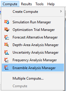
- From the top menu bar, select Compute | Ensemble Analysis Manager.
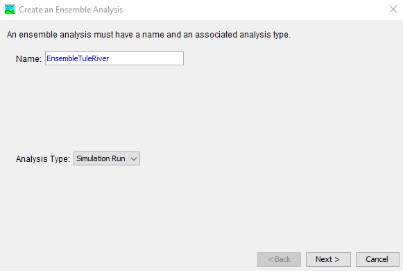
- Select New... and name the analysis EnsembleTuleRiver. Select Simulation Run as the analysis type and then select Next.
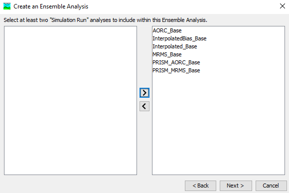
- All of the simulation runs that have been previously created are available for selecting as part of this ensemble analysis. Select them all by moving them from the left window pane to the right window pane. Select Next and then Finish.
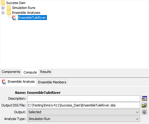
Now that the ensemble analysis has been created, we can select and further refine it by selecting the Compute tab of the Watershed Explorer.
Note:
Depending on the detail and number of simulation runs that are included within an ensemble analysis, the file size of the HEC-HMS project can quickly balloon. An important way to keep computation time and file sizes more manageable is to only generate the results output that you as the user are interested in.
To select the time-series results output that you wish to generate during a compute, select the output gear icon.

For this analysis, we are interested in computing all of the available time-series results for MF_TuleR_S20 since this subbasin is higher up in elevation and likely will have meaningful snowmelt results to analyze. We are also interested in both Outflow and Cumulative Outflow results for the ReservoirInflow element. Lastly, we would like to analyze Cumulative Precipitation and Moisture Deficit at subbasin TuleR_S10 which is located at a lower elevation in proximity to the watershed outlet. Include only these eleven time-series results by checking the box next to them as seen below. Click Save and then Close to exit the window.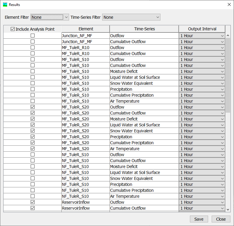
Note:
When the above output control table is populated, all of the ensemble analysis members are iterated over. Only the elements and time-series that are available in ALL of the members will be available for selection within the table. If, for example, an element is present in some of the members (simulation runs) but not all of them, it will not be available for analyzing within the ensemble analysis compute.
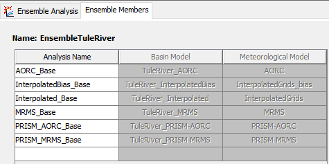
If needed, simulation runs can be removed and/or added to the ensemble analysis via the table located on the Ensemble Members tab. We wish to include all six of the previously selected simulation runs so no further refinement is necessary.
- Finally, let's compute the Ensemble Analysis. Select EnsembleTuleRiver in the compute dropdown and then click the Ensemble Analysis icon to begin the compute.

During the Ensemble Analysis compute, each of the base simulation runs will first be computed and then the final ensemble results will be aggregated.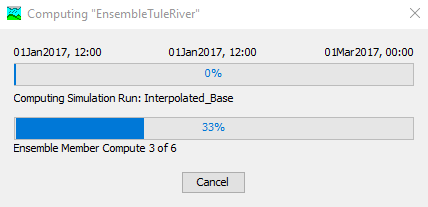
View the Ensemble Analysis Results
- The Ensemble Analysis results can be accessed in the Watershed Explorer via the Results tab. Results should only be available for the elements and time-series that you selected earlier. Expand the results for the MF_TuleR_S20 subbasin element.
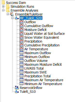
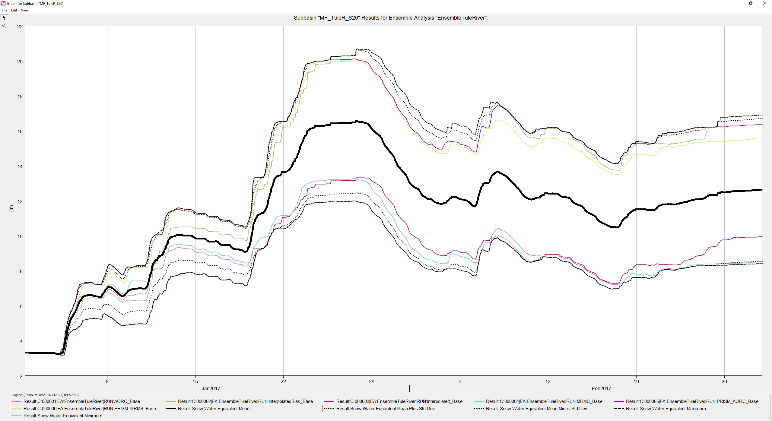
- Select the Snow Water Equivalent (SWE) plot node to see a time-series plot of the results. In addition to seeing the traces from each of the six simulation runs, you will also notice aggregated time-series results including SWE Maximum, Minimum, Mean, and +/- One Standard Deviation. Selecting an individual time-series within the legend will bolden it in the plot for easier visualization.
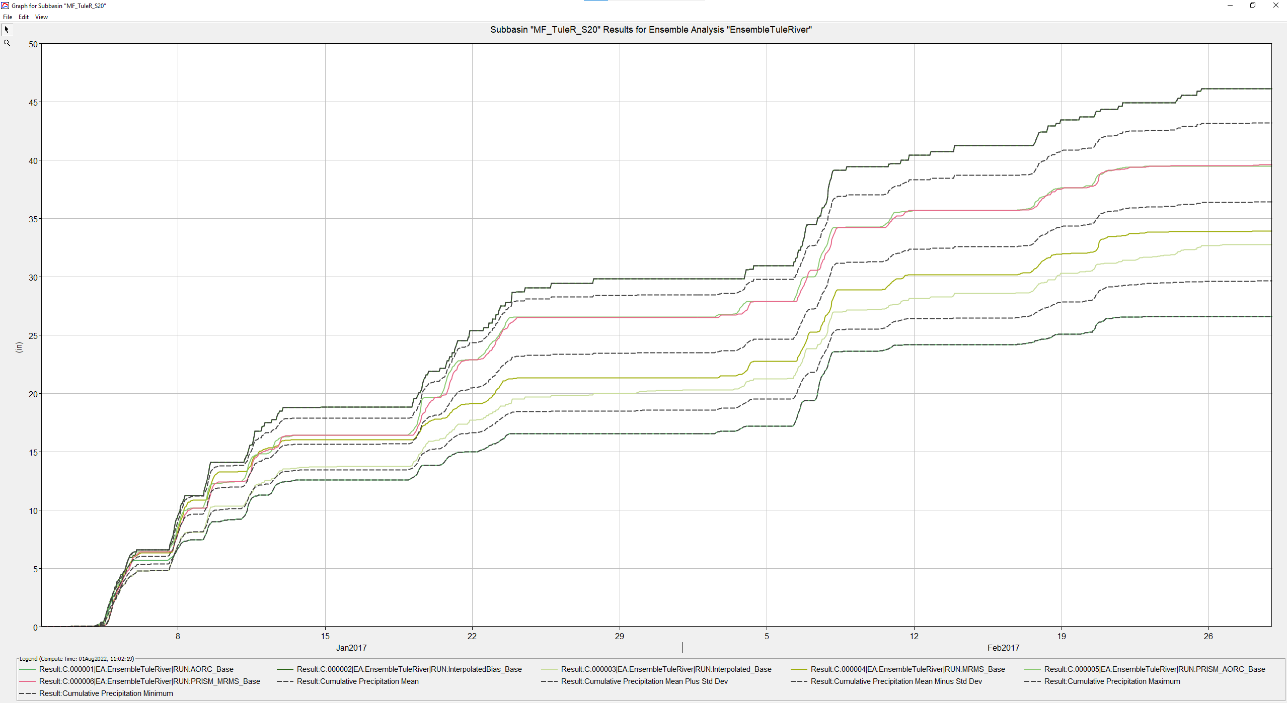
Select the Cumulative Precipitation plot node to view the results. At the end of the two month simulated time period, do the cumulative precipitation results vary?
The total accumulated precipitation amounts do vary significantly. The interpolated bias precipitation led to the highest accumulated amounts (~46 inches) whereas the base AORC precipitation led to the lowest accumulated amounts (~27 inches). Sources of gridded precipitation (and other boundary condition data), are often a significant source of uncertainty.
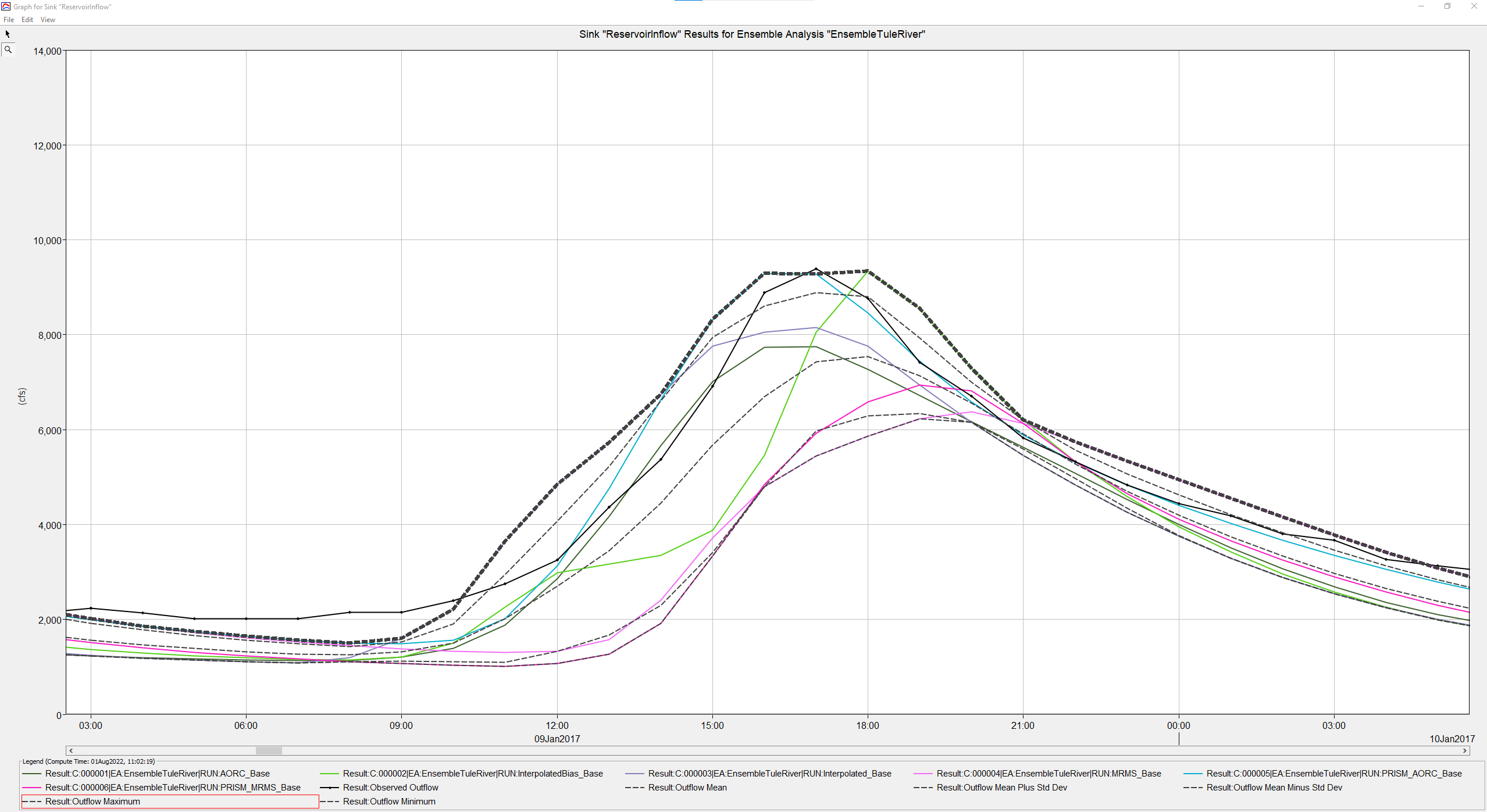
If a basin element has an observed time-series associated with it, the observed data should be shown on the results plots. Expand the results for the ReservoirInflow element and select the Outflow plot to open it. Use the magnifying glass to zoom into the peak of the hydrograph that occurred on the afternoon of 09 January 2017. Which of the time-series traces best reflects the observed peaks? What about the observed rising and recession limbs?
The interpolated bias simulation results, the PRISM corrected AORC simulation results, as well as the outflow maximum time-series statistics all do a good job of matching the observed peak flows. For the rising limb, the AORC simulation results most closely mirror the observed data. For the receding limb, the PRISM corrected AORC simulation results somewhat reflect the observed data.
