Download PDF
Download page Correcting Precipitation Volume with the Normalizer Utility.
Correcting Precipitation Volume with the Normalizer Utility
It is sometimes the case when modeling with gridded precipitation data that the data product that best captures the temporal distribution of rainfall does not best capture the cumulative volume of precipitation. The Normalizer Tool within HEC-HMS can be used to create a normalized precipitation grid that captures the temporal variability of one gridded dataset but the cumulative volume of another gridded dataset. For example, radar data collected at an hourly timestep may adequately capture temporal variability over the simulation window, but a grid based on gage data collected at a daily timestep may better capture the total volume of rainfall. For a detailed example showing how the Normalizer Tool computes the normalized grid, see the Normalizer User's Manual Reference.
This tutorial demonstrates how gridded, National Centers for Environmental Protection (NCEP) Stage IV precipitation data can be corrected, or "normalized" using gridded, PRISM data within HEC-HMS 4.9. This tutorial will also show simulated runoff volume before and after normalization using an existing model of the Sonoma Creek watershed. At the end of the tutorial, there is an additional section showing how the normalized grid values are computed.
Initial project files
Sonoma Creek HMS model: Sonoma_Creek_Initial.zip
Precipitation Data:Precip_Data.zip
Note that files are provided in a compressed folder and must be unzipped.
Inspect Grid Data
Prior to normalizing the precipitation data, it is important to inspect the grid datasets to make sure they have the same units, data type, cell size, and projection. Both grids must also share the same lower left cell and grid extents, such that every cell covers the exact same geographic area in each grid. To view this information, open the gridded datasets in the "Precip_Data" folder in HEC-DSSVue, select a grid file, right-click, and select "Edit." As shown in the images below, the Stage_IV and PRISM grids both share the same Grid Type, Data Units, Data Type, Lower Left Cell, Grid Extents, Cell Size, and Spatial Reference. If any of these parameters differ between the two grids, the grids must be preprocessed such that these parameters are identical.
Source Grid: Stage IV grid (captures temporal variability but lacks correct volume)
Normal Grid: PRISM grid (lacks temporal detail but better captures cumulative volume over the simulation window. The Normals Grid is used to adjust the Source Grid)

The precipitation grids used in this tutorial were converted to HEC-DSS format using the Gridded Data Import Wizard in HEC-HMS. There are several tutorials showing how to use this tool with different gridded data products.
Using the HEC-HMS Normalizer Tool
The Normalizer Tool in HEC-HMS guides the user through the process of normalizing an existing, "source" grid using another, "normal" grid to create a corrected, or "normalized" grid. To launch the Normalizer Tool, select Tools | Data | Normalizer…. The Grid Normalizer Wizard appears.

Select Grid Files
Under Select Source File, click the folder icon, navigate to the "Stage_IV.dss" file in the "Precip_Data" folder, select the file, and click Open.
In the Select Source Grids panel, select the grids for the time period 25DEC2005:1200 through 10JAN2006:1200. When the grids are highlighted, press the right arrow in the center of the dialog box to move the files to the second panel and select Next.
The source grids were selected to begin at 1200 hours because the PRISM data is recorded at 1200 hours. If, for example, the normal grids began at time 0000, the first source grid should begin at time 0000.
In the next window, under Select Normal File, click the folder icon, navigate to the PRISM.dss file in the Precip_Data folder, select the file, and click Open.
In the Select Normal Grids panel, select the grids for the time period 24DEC2005:1200 through 10JAN2006:1200. When the grids are highlighted, press the right arrow in the center of the dialog box to move the files to the second panel and select Next.
The time periods for the source and normal grids should match. In this example, the normal grids begin at 1200 and end at 1200 the next day. Therefore, the first source grid begins at 1200, and the last source grid ends at 1200.
Set Normalization Period and Interval
After selecting the source and normal grids, the user is prompted to enter a Normalization Period and Normalization Interval. The Normalization Period defines the time window that the normalized grids should be created for. The Normalization Interval sets the time window that the source and normal volume should be accumulated over during the normalization computation. A simple example showing how the Normalization Interval affects the computed grid cells is shown in Part 2b: Selecting a Normalization Interval. 
Set the Start and End times for the Normalization Period equal to the start and end times of the source grids (25 Dec, 2005: 1200 – 10 Jan, 2006: 1200). Enter dates in mm/dd/yyyy format. Set the Normalization Interval to 1 day. Then, select Next.
It is very important to select a start time for the Normalization Period that corresponds to the start time of the normal grids. It is also important to select a Normalization Interval such that a whole number of normal grids make up one interval.
If for example, the normal grids span 0600-1800 but the Normalization Interval is 1200-1200, some data will not be included in the normalization computation for a given interval, as shown below:
Set File Destination for Normalized Grids
In the next window, select the location to store the normalized grids. Either select the folder icon, navigate to a location, enter a file name, and select Open, or enter a pathname directly into the text box.
After selecting the filename and location, the user is prompted to enter the A-, B-, and F-Parts of the normalized grids. Note that the C-, D-, and E-Parts of the pathnames use the wildcard asterisk because the program automatically names these parts based on the type and timestep of the data. Enter "Stage IV Norm" for the F part and select Next. After selecting "Next" the Normalizer Tool computes the normalized grids and exports them to the user-defined location. The computations are complete when the status bar reaches 100%. After the computations are complete, the tool can be restarted or closed.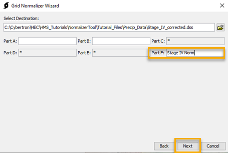
Using the Normalized Grid in HEC-HMS
This tutorial uses an HEC-HMS model (version 4.9) of the Sonoma Creek watershed in northern California. The Sonoma Creek basin model consists of one subbasin and one outlet node with observed streamflow data. After creating and running a simulation using the normalized grid, the results will be compared to a simulation using the original Stage IV data and a simulation using the original PRISM data.
Create New Grid Data Object
A parameter grid must be created to store the normalized grid data. Within HMS, select Components | Create Component | Grid Data… to generate a parameter grid. Provide a recognizable name and description of what the data represents. The data type should be Precipitation Gridsets. Click Create to add the new precipitation grid to the HMS model.
Select Previously Created HEC-DSS File and Part Names
The Grid Data Object created in the previous step is now available within the Grid Data | Precipitation Gridsets tree in HMS. Select the "Stage_IV_corrected" grid created in the previous step. The data source should be set to Single Record HEC-DSS. The DSS Filename should be the pathname of the "Stage_IV_corrected.dss" file and a single pathname from the DSS file needs to be selected. Any pathname within the DSS file can be selected.
Configure Meteorological Model
Create a new meteorological model by selecting Components | Meteorological Model Manager | New… Provide a name and description for the new meteorological model. Click Create when finished entering a name and description.
Select the "Stage_IV_corrected" meteorological model from the Meteorological Models tree. Select the "Gridded Precipitation" option within the Precipitation dropdown menu and set the Replace Missing option to "Set to Default." This allows the simulation to continue if a timestep with missing data is encountered.
Click the "Basins" tab of the "Stage_IV_corrected" meteorological model and ensure the basin model that will be used for the simulation is set to "Yes."
Within the "Stage_IV_corrected" meteorological model, highlight the Gridded Precipitation icon. Select the "Stage_IV_corrected" option within the Grid Name dropdown menu.
Create a Simulation Run
Set up a simulation run that uses the normalized grid, a basin model, a meteorological model, and control specifications. For this exercise, the existing basin model and control specifications will be used rather than creating separate model components. Select Compute | Create Compute | Simulation Run… to access the Create a Simulation Run Wizard.
Provide a descriptive name for the simulation run. Click Next."

Select a basin model to use with the simulation run. In this case, use the existing basin model. Click Next.
Select the meteorological model that uses the normalized data. Click Next.
The final step is the select the control specification. For this case, the existing "Dec_2005_Jan_2006" control specifications can be used. Click Finish. The simulation run is now created and ready to use.
Compute the Simulation
Select the simulation run that was created in the previous step from the Compute dropdown box. Press the compute button to perform a simulation. In this example, the simulation computed in less than 10 seconds.
Visualize Results
The initial Sonoma Creek HEC-HMS model contains a simulation run using the original, uncorrected Stage IV data (Dec2005_Jan2006_base) and a simulation run using the PRISM data (Dec2005_Jan2006_PRISM). Before viewing the results of the normalized simulation, view the results of the initial simulations at the "SonomaCr" node by expanding each simulation in the "Results" tab of the model interface, expanding the "SonomaCr" element, and selecting "Graph."
The simulation results show the hourly Stage IV data effectively captures the timing of the flood peaks, but the magnitude of runoff is significantly less than what was observed at the gage. A greater volume of runoff is generated when the daily PRISM data is used, but the timing and shape of the hydrograph do not match the observed data well.

To view the difference in cumulative precipitation volume between the Stage IV and PRISM datasets over the simulation window, expand the "SonomaCr_S10" basin element for the "Dec2005_Jan2006_base" and "Dec2005_Jan2006_PRISM" simulations. Then, hold the CTRL key, select "Cumulative Precipitation" for each simulation, and select the plot icon on the toolbar.

The PRISM data accounted for over twice as much precipitation volume as the Stage IV data during the simulation period.
The above plot illustrates a common issue with using radar-generated precipitation grids in the western United States. While it is not clear exactly why there is such a large difference in accumulated volume between the two datasets, one explanation could be radar beam blockage from mountainous terrain. Since PRISM data is gathered from a wide range of monitoring networks and applies a more sophisticated quality control system, it may capture the total volume of precipitation more accurately.
Now, add the cumulative precipitation volume for the normalized grid to the plot by expanding the "SonomaCr_S10" basin element for the normalized simulation, holding the CTRL key, selecting "Cumulative Precipitation" for all three simulations, and selecting the plot icon on the toolbar. Note how the cumulative precipitation for the normalized grid now closely follows the cumulative precipitation for the PRISM dataset. data")
To view the simulated runoff hydrograph at the Sonoma Creek gage using the normalized grid, expand the "SonomaCr" element within the normalized simulation and select "Graph." The simulated runoff using normalized precipitation grid closely matches both the timing and the magnitude of the observed data.
Final project files
Final HMS Project:Sonoma_Creek_Solution.zip