Download PDF
Download page Time of Concentration and Storage Coefficient Impacts to the Hydrograph.
Time of Concentration and Storage Coefficient Impacts to the Hydrograph
Last Modified: 2025-01-29 17:10:27.805
This tutorial evaluates impacts of Clark unit hydrograph parameters on the hydrograph response.
Software Version
HEC-HMS version 4.13 beta 4 was used to create this example. You can open the example project with HEC-HMS 4.13 or a newer version. Downloads are available here: https://www.hec.usace.army.mil/software/hec-hms/downloads.aspxProject Files
Continue using the project files from the previous Estimating Time of Concentration & Storage Coefficient tutorial.
Overview
This tutorial will compare how the computed hydrograph changes with adjustments to your time of concentration and storage coefficient parameters. We will be creating four additional basin models and simulations runs to compare results.
Create Four Additional Basin Models
- Create four additional Basin models.
- In the Components tab under Basin Models, right click on Sep2018 and select Create Copy.

- Name the copied basin model Sep2018 - double Tc.

Create three more copies of the Sep2018 basin model and name it Sep2018 - half Tc, Sep2018 - double R, Sep2018 - half R. You should now have five basin models listed in the project.

- In the Components tab under Basin Models, right click on Sep2018 and select Create Copy.
- Create a simulation run for each of your new basin models.
- Navigate to your Compute tab, expand the Simulation Runs folder by clicking on the + sign, right click on Sep2018 Simulation Run, and select Create Copy.

- Name the copied simulation run Sep2018 - double Tc. Select this simulation run and change in the Basin Model to Sep2018 - double Tc.

- Create another copy of the simulation run and name it Sep2018 - half Tc. Repeat the previous step above and select Sep2018 - half Tc Basin Model for the Sep2018 - half TC simulation run.
- Repeat the above steps and create two more simulations that use the Sep2018 - double R and Sep2018 - half R basin models.
- Navigate to your Compute tab, expand the Simulation Runs folder by clicking on the + sign, right click on Sep2018 Simulation Run, and select Create Copy.
Adjust the Time of Concentration
Pro Tip
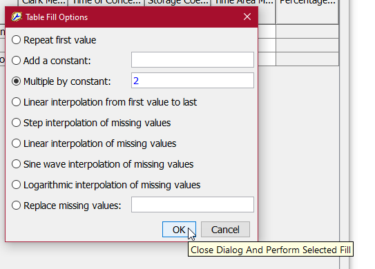
A fast way to make multiplicative adjustments to a large number of parameters is to use the Global Editor table's "Fill" function. Open a Global Editor for the Clark UH by clicking on the basin model and using the Parameters > Transform > Clark Unit Hydrograph menu option.
Then, in the table, select the values you want to change (for example, all the Storage Coefficient value), right click on them, and choose the "Fill..." menu option.
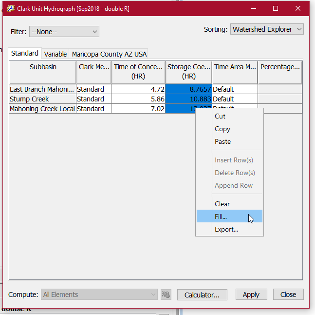
Then in the Table Fill Options dialog that appears, choose the "Multiple by constant" option and enter the desired value (such as 2, for a doubling.)
- Adjust the time of concentration for the two additional basin models.
- Navigate back to the Components tab. Select the Sep2018 - double Tc basin model and expand the element tree. For each subbasin, double the time of concentration while keeping the storage coefficient values the same.
- Do the same for the Sep2018 - half Tc basin model but divide your time of concentration for each subbasin by half.
- In the Compute tab (or using the compute toolbar) run the Sep2018 - double Tc and Sep2018 - half Tc simulations.
- Plot the Outlet Outflow for original and adjusted Tc simulations.
- Expand the Mahoning Creek at Punx Gage element for each of the Time of Concentration simulations and the original Sep2018 simulation. Click and hold the Ctrl button and select Mahoning Creek at Punx Gage for each simulation to plot the Outflow graphs together. You should three Outflow graphs plotted.

- Expand the Mahoning Creek at Punx Gage element for each of the Time of Concentration simulations and the original Sep2018 simulation. Click and hold the Ctrl button and select Mahoning Creek at Punx Gage for each simulation to plot the Outflow graphs together. You should three Outflow graphs plotted.
- Click on the View Graphs for Selected Elements button to display the plots in a separate window. Zoom into the flood event as shown in the figure below.


- Plot the Outlet Outflow for original and adjusted Tc simulations.
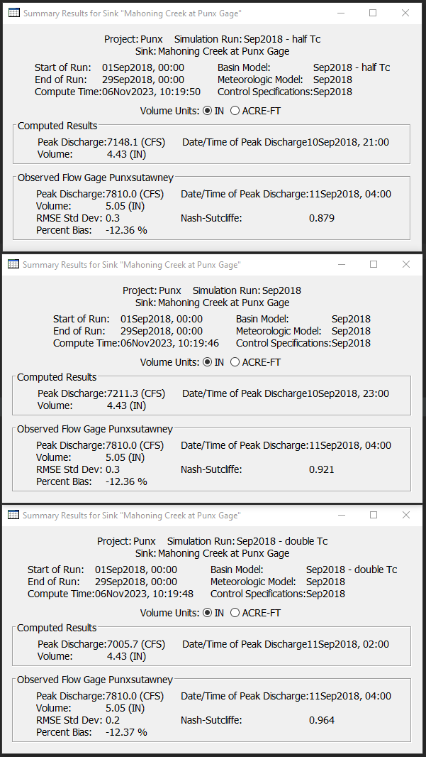
- In the Summary Results, note the difference in Date/Time of Peak Discharge.
Adjust the Storage Coefficient
Similarly, now we will review how changes to the Storage Coefficient change the computed hydrograph.
- Adjust your storage coefficient for the two basin models.
- Navigate back to the Components tab. Select the Sep2018 - double R basin model and expand the tree. For each subbasin, double the storage coefficient while keeping the time of concentration values the same.
- Do the same for the Sep2018 - half R Basin model but divide the storage coefficient for each subbasin by 2.
- In the Compute tab (or using the compute toolbar) run your simulation for Sep2018 - double R and Sep2018 - half R.
- Plot the Outlet Outflow for original and adjusted R simulations.
- Expand the Mahoning Creek at Punx Gage element for each of the Storage Coefficient simulations and the original simulation. Click and hold the Ctrl button and select Outflow for each simulation to plot the outflow graphs together. Click the View Graph button to see a larger plot and then use the magnify button and zoom into the hydrograph from September 9 - 13.

- Expand the Mahoning Creek at Punx Gage element for each of the Storage Coefficient simulations and the original simulation. Click and hold the Ctrl button and select Outflow for each simulation to plot the outflow graphs together. Click the View Graph button to see a larger plot and then use the magnify button and zoom into the hydrograph from September 9 - 13.
Bonus:
- If time allows, try other combinations of Tc and R and see how they change the simulated hydrograph. Adjust Tc and R to match the observed hydrograph as well as possible.
- Try another synthetic unit hydrograph method (SCS or ModClark) and attempt to calibrate the model.

Questions
What happens when you change your time of concentration in terms of hydrograph peak, shape, and timing? In general, what might cause the time of concentration to be shorter or longer for any watershed? How did the Tc changes compare to the observed hydrograph?
The time of concentration is the time it takes for water to travel from the most remote point in the watershed to the watershed outlet (pourpoint). By reducing the time of concentration, the hydrograph arrives at the outlet sooner. By increasing Tc, you see the hydrograph shift to the right meaning water arrives at the watershed outlet later. The hydrograph peak and shape do change slightly with changes to Tc but the most apparent changes is the timing of the hydrograph. Looking back at the initial Tc equation, the longest flow path, centroidal flow path, and slope are basin parameters that could affect the time of concentration. Other potential factors could be the basin and channel roughness, channel shape, or urbanization. By increasing Tc, the simulated hydrograph appears to match the observed hydrograph much better.
What happens when you changed the storage coefficient in terms of hydrograph peak, shape, and timing? How does increasing or decreasing R compare to the observed hydrograph?
The storage coefficient is a representation of temporary water storage. By reducing "R", the hydrograph shape "narrows" (the rising limb and recession limb have a steeper slope) causing the peak value to increase while also reducing the time to peak. By increasing R, the hydrograph shape "flattens" or attenuates which reduces the hydrograph peak and extends the recession limb of the hydrograph later in time. Reducing R narrows the shape of the simulated hydrograph and increases the peak above the observed hydrograph. Increasing R attenuates the hydrograph such that the hydrograph shape matches pretty well but the peak value is much lower compared to the observed hydrograph.
This tutorial concludes the Estimating Clark Unit Hydrograph Parameters tutorial group.