Applying the Frequency Storm Met Model in HEC-HMS

Last Modified: 2023-06-30 07:10:07.843

Software Version

HEC-HMS version 4.11 beta 9 was used to create this tutorial. You will need to use HEC-HMS version 4.11 beta 9, or newer, to open the project files.

Suggested Time

This workshop should take approximately 1-hour to complete.

Project Files

Download the initial project files here: 

Frequency_Storm_HMS_Project_Initial.zip

Background

The Frequency Storm meteorologic model is designed to produce a synthetic storm from statistical precipitation data. A fundamental characteristic of this method is that it uses the "balanced hyetograph" approach. Typically, the precipitation data are stored and retrieved in the form of maps, where each map shows the expected precipitation depth at a given point for a storm of specific duration and exceedance probability. The frequency storm meteorologic model is designed to use data collected from the maps along with other information to compute a hyetograph for each subbasin. 

Frequency based precipitation information is often available for point, or precipitation gage, locations. When applying point precipitation to a watershed, area-reduction factors are required to reduce the point precipitation to an average depth that occurs over the watershed. The general pattern observed from historic storms is that the rainfall magnitude decreases as storm area increases. Therefore, area-reduction curves are a required component to account for the storm, or watershed, area.

HEC-HMS can automatically apply an area-reduction factor based on the storm area entered in the frequency storm meteorologic model. However, the area-reduction curves that are hardcoded into HEC-HMS are from Technical Paper No. 40 and may not be accurate for watersheds larger than 400 square miles. The TP40 reduction curves were developed using only drainage areas of 400 square miles or less so the curves flat line and use similar reduction factors for storm area over 400 square miles. Logically, we know that as storm areas increase in size, the reduction factor should continue to decrease. Also, there is evidence that area-reduction varies across the country. For this reason, a new User-Specified option exists in HEC-HMS where modelers can create and specify their own area-reduction curves specific to their area of interest.

In this workshop, you will learn how to create site specific area-reduction curves. By applying site specific area-reduction factors into HEC-HMS, you can improve the accuracy of the area-reduced rainfall depths for your local watershed. A secondary component to this workshop is application of the Depth-Area Analysis simulation type in HEC-HMS. The Depth-Area Analysis allows the modeler to choose multiple points within a basin model and the program will automatically apply appropriate area-reduction factors when simulating the runoff response to each of the defined points (think of the analysis as multiple simulations within the analysis).

The following major tasks will serve as an outline for this workshop:

1. Gather Historic Storm Data.
2. Create a Storm Specific Depth-Area-Reduction Curves.
3. Gather Precipitation Frequency Depth-Duration Data from NOAA Atlas 14.
4. Create a Frequency Storm in HEC-HMS.
5. Compare Results.
6. Extra Task 1 - Use Area-Reduction Information from a Second Historic Storm in HMR 51.
7. Extra Task 2 - Create a Depth-Area Analysis Simulation and Evaluate Results.

Goals

In this workshop, you will:

• Create site specific area-reduction curves.
• Apply the Frequency Storm meteorological model to estimate frequency flows at a point of interest for the 1/100 annual exceedance probability (AEP).
• Investigate the impact that area-reduction curves have on computed flow results.
• Apply the Depth-Area Analysis compute type in HEC-HMS.

Data

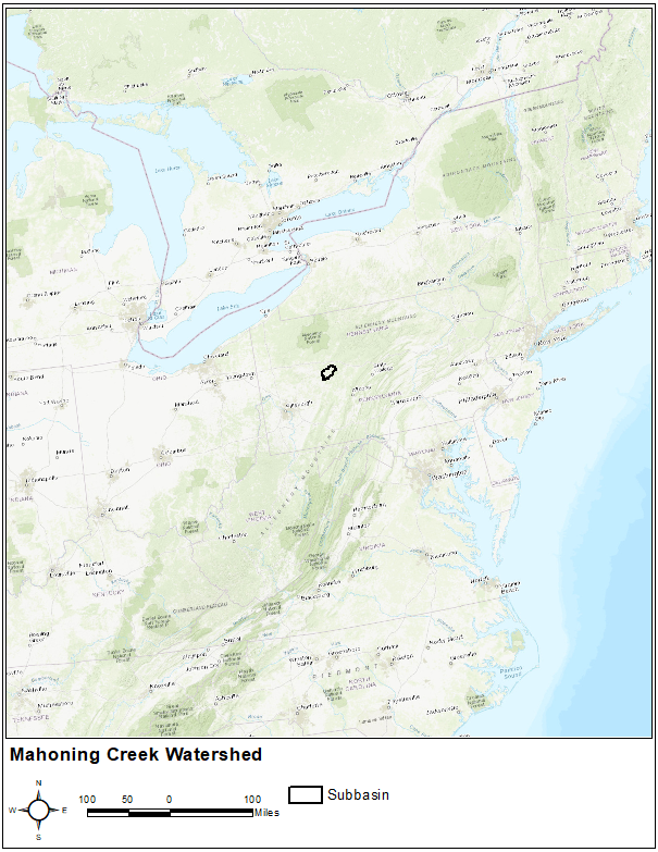
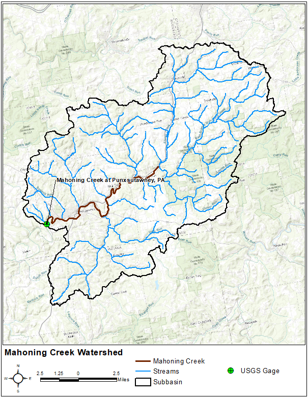
You will be using an HEC-HMS model of the Punxsutawney watershed for this workshop. The basin model has been created for you. This watershed is located in Pennsylvania and is approximately 158 sq. mi. A location map and delineation map can be seen below.

1. Gather Historic Storm Data

For this workshop, depth-area-duration information from historic storms in NOAA’s Hydrometeorological Report No. 51 (HMR 51) will be used. The storms contained in HMR 51 were influential in setting the level of Probable Maximum Precipitation (PMP) for the Eastern U.S. 

1. Go to NOAA’s web page that houses current NWS PMP documents (https://www.weather.gov/owp/hdsc_pmp).
2. Considering our watershed location, select the HMR 51 document link.
3. The figure below shows the locations of the more influential storms used to develop PMP index maps. This figure was copied from HMR 51.
   
4. For this workshop, one sample storm will be evaluated, but in reality you may want to use multiple historic storms to develop area-reduction information. We will be using storm number 76. Make note that this is not the closest storm to our watershed, but for workshop purposes, this storm is used to show a larger impact on the area-reduction curves.
5. Starting on page 79 in HMR 51 (pdf page 87) are the depth-area-duration tables for major storms, listed chronologically. Scroll to storm number 76.
6. Next you would manually transfer the depth-area-duration information to an Excel sheet. This step has been completed for you.
7. Open the Excel file named area_reduction_curves_initial.xlsx. You should pay attention to two tabs, HMR 51 and TP40.  The TP40 tab contains the area-reduction values that are hard-coded into HEC-HMS. The HMR 51 tab will be used to create area-reduction factors for storm number 76.

2. Create Storm Specific Depth-Area-Reduction Curves

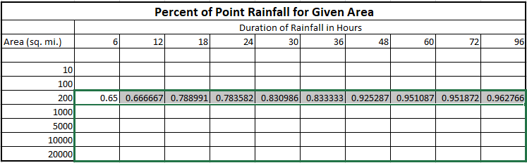
Using the depth-area-duration information in HMR 51, storm specific area-reduction curves will be computed. Ratios will be computed for this historic event based on the 10 square mile depths (assuming the 10 square mile depth is the point rainfall depth). A table for this purpose, Percent of Point Rainfall for Given Area, has been created for you to the right of the original table.

1. Using Excel functions, populate the new table by dividing each cell in each column by the 10 sq. mi. depth (the top cell.) The top cell in each column should equal 1 and each succeeding cell will be less than 1. For example, the formula for cell P:10 should be C:10 / C:8 (3.9 inches / 6 inches). The ratio should equal 0.65. For storm 76, the 200 square mile depth was 65 percent of the 10 square mile depth.

   

   Absolute Cell References ($) in Excel

   In Excel, the '$' symbol can be used to specify an absolute cell reference. In this case, the “Percent of Point Rainfall for Given Area” table values are all based on the 10 sq. mi. depth located on row 8. To hold row 8 constant, an absolute cell reference can be used. For example, the formula for cell P:10 can be entered once as C:10 / C:$8. Then, click in the P:10 cell to select it and drag the bottom right portion of the cell towards the right all the way to Y:10. This will fill out the entire row. With the entire row still selected, the bottom right portion of the selected row can be dragged down (and up) to quickly fill out the entire table. 

   

2. Compare the new area-reduction curves against those from TP40. In this workshop, the 6 hour and 24 hour curves will automatically populate in the included chart (light and dark blue lines), as shown below. These two curves were chosen to compare to the TP40 curves that are hardcoded into HEC-HMS.

Two charts are included on the HMR 51 Excel sheet tab. The top chart only includes areas up to 400 square miles to show detail for smaller watersheds. The bottom chart extends out to 20,000 square miles to show that the reduction from storm 76 continues for areas greater than 400 square miles. As you can see below, the area-reduction curves from HMR 51 storm 76 are significantly lower than the TP40 area-reduction curves.

3. Gather Precipitation Frequency Depth-Duration Data from NOAA Atlas 14

NOAA Atlas 14 provides point precipitation frequency estimates.

1. Go to NOAA’s Precipitation Frequency Data Server web page (https://hdsc.nws.noaa.gov/hdsc/pfds/) and click on the state of Pennsylvania (PA). 
2. Change the Time series type option from Partial Duration to Annual Maximum.
3. Type in “Punxsutawney, PA, USA” as the location (use option C to define the location by address).
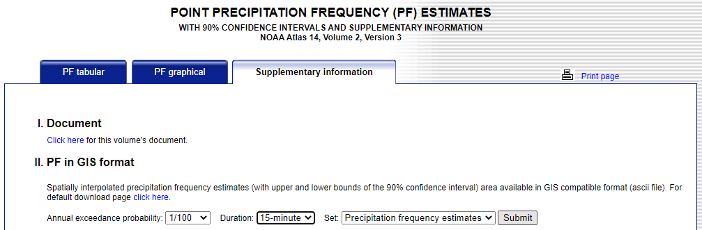
4. The frequency-depth-duration table will populate below the map as shown in the below figure.
   
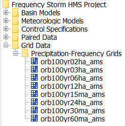
5. In this workshop, the 1% frequency storm will be simulated. The frequency-depth values from the 1/100 annual exceedance probability column COULD be copied and pasted manually into the Frequency Storm Component Editor as seen in the figure associated with Task 4, Step 8 below. However, HEC-HMS now has the ability to ingest NOAA Atlas 14 precipitation-frequency grids directly. These grids can be found on the Supplementary Information tab. For this workshop, we are interested in the 1/100 annual exceedance probability and the 15-min, 30-min, 1-hour, 2-hour, 3-hour, 6-hour, 12-hour, and 1-day durations. Each of these grids have already been downloaded for you and are located in the data folder in your HEC-HMS project directory.
   
6. There is now a tool to rapidly import NOAA Atlas 14 precipitation-frequency grids into HEC-HMS. Open the Frequency_Storm_HMS_Project.hms project file in HEC-HMS. To access the Precipitation Frequency Grid Importer, click File | Import | Gridded Data | Precipitation Frequency.
7. Click the directory button and navigate to the data folder in your project directory. Select all of the precipitation frequency grids as seen below and then click Open. 
   
8. The importer dialog should now look similar to the below figure. Leave the other columns (Name, Units, and Unit Scale Factor) set to the defaults. NOAA Atlas 14 values are stored with a unit scale factor of 1000.0 in order to remove decimal places for file size efficiency.
   
9. Click Import. A Grid Data object should have been automatically created from each NOAA Atlas 14 input file as seen below.
   

Balanced Hyetograph

The Frequency Storm met model utilizes what is commonly referred to as the "balanced hyetograph" approach. This method ensures that the appropriate intensity for each duration is maintained throughout the total storm. So if the goal were to build a 1/100 AEP 24 hour synthetic storm using the balanced hyetograph approach, the 1/100 1 hour duration, 1/100 2 hour duration, 1/100 3 hour duration, etc. would all be contained within the storm hyetograph in a neat, nested manner.

As an example, let's assume that the following depths were retrieved from NOAA Atlas 14 for the 1/100 AEP event at a given location.

	1-hr	2-hr	3-hr	6-hr	12-hr	24-hr
Depths (inches)	3.62	4.67	5.37	6.59	7.86	9.18

A balanced hyetograph built from the above depth information might look like the below figure. If all 24 of the time blocks were added up, the depth would total to 9.18 inches. 

The balanced hyetograph in this example has not been reduced. Area-reduction factors would need to be applied to each depth at each duration when computing a simulation. You will learn how to apply area-reduction functions in the following section of this workshop.

4. Create a Frequency Storm in HEC-HMS

Now that all the necessary data have been gathered, the next step is to create a frequency storm within HEC-HMS. A calibrated basin model has been created for you. For results comparison later on, a meteorologic model named TP40 has also already been created for you and is shown with the typical NOAA Atlas 14 depth input in the figure below. The frequency storm option has been chosen with the following parameters: intensity duration of 15 minutes, area reduction using TP40 TP49 curves, storm duration of 1 Day, storm area of 158 square miles (the area of our watershed). Depths have been entered straight from Atlas 14. During the simulation run using this meteorologic model, HEC-HMS automatically reduced the precipitation depth values according to the hard-coded TP40 area-reduction curves and the input storm area of 158 square miles.

In this task, you will create a new meteorologic model similar to the TP40 meteorologic model above. However, instead of the TP40 area-reduction curves, you will apply the area-reduction curves from HMR Storm 76 data that were developed in Task 2.

1. Create a new meteorologic model. Name it HMR Storm 76.
2. In the Watershed Explorer, select the new meteorologic model you just created to open the component editor.
3. Change the Precipitation option to Frequency Storm. Make sure the Unit System is set to U.S. Customary.
4. Click the Basins tab. Change the Include Subbasins option from No to Yes for the Base 1% basin model.
5. Now click on Frequency Storm under your HMR Storm 76 meteorologic model.
6. Make sure the Storm Duration option is set to 1 Day. Change the Intensity Duration option from 5 Minutes to 15 Minutes.
7. Change the Area Reduction option to User-Specified, then the Storm Area option to User-Specified, and then enter a Storm Area of 158 square miles.
8. Click Save. The Frequency Storm component editor should now look identical to the below figure.
   
9. To automatically calculate and populate the depth column, click the blue calculator button. Select the appropriate grid for each duration as seen below, then select Calculate. Next select OK to populate the depth column with the calculated results.
   
10. Next, we need to load the previously calculated area-reduction curves (from the Excel spreadsheet, HMR51 tab) into HEC-HMS. Go to Components | Paired Data Manager. For Data Type, select Area-Reduction Functions and then click New. Name it 6hr_ARF_76 and click Create.
11. In the watershed explorer, navigate to Paired Data | Area-Reduction Functions. Select the 6hr_ARF_76 and then select the Table tab in the component editor. This watershed is 158 square miles, so only areas of 10.0, 100.0, and 200.0 need to be listed in the table. In the Excel spreadsheet HMR51 tab, find the appropriate 6-hour reduction factor values from the table Percent of Point Rainfall for Given Area and copy them to the paired data table in HEC-HMS as seen below.
    
12. Repeat the prior two steps to create a 12hr_ARF_76 and a 24hr_ARF_76 with areas of 10.0, 100.0, and 200.0 sq. mi. and reduction factor values from the Excel spreadsheet HMR51 tab.
13. Now navigate back to the Frequency Storm Component Editor in the watershed explorer by clicking on Frequency Storm under the HMR Storm 76 meteorologic model.

14. Under the Area-Reduction Function column, associate the 6hr_ARF_76 with the 15 Minute to 6 Hour durations. Associate the 12hr_ARF_76 with the 12 Hour duration and the 24hr_ARF_76 with the 1 Day duration. Your fully parameterized component editor should reflect what is shown in the figure below.
    

    

    HMR 51 Historical Storms

    While still useful, HMR 51 is an antiquated document. The depth-area-duration tables were developed from storms that occured in the 1970s and prior. Storm data back then were not as comprehensive as they are now; as a result, most of the storms only have data recorded in 6-hr intervals. As demonstrated in the Percent of Point Rainfall for Given Area table in the Excel spreadsheet, duration is typically inversely related to the amount of reduction. So, in this example, applying a 6-hr area-reduction curve to smaller durations such as the 1 Hour is not ideal. 1 hour point precipitation values should typically be reduced more than 6 hour point values, but in this case it is the best we can do given the constraints of the available data for this historical storm.

    Today, gridded storm data for more recent storm events are becoming increasingly reliable with temporal resolutions typically available in at least one hour intervals. When developing area reduction curves, it is highly recommended to look at multiple historical storm events that are similar in magnitude and duration to what you are trying to model. Tools such as HEC-MetVue exist that can rapidly ingest gridded datasets and create depth-area-duration tables that can be used to develop area-reduction factors for your study area. For a tutorial and guide on this topic, see the following link: Creating Depth-Area Reduction Curves from Gridded Precipitation Data.

15. Lastly, create a new simulation run.
16. Enter the name HMR Storm 76. Choose the Base 1% basin model. Choose the HMR Storm 76 meteorologic model. Choose the Hypothetical control specifications. Click Finish.
17. Go to the Compute tab in the Watershed Explorer. Right click on the HMR Storm 76 simulation and click Compute.

5. Compare Results

1. Go to the Results tab in the Watershed Explorer.
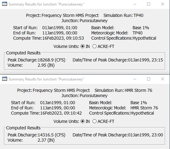
2. Compare the Global Summary tables for the TP40 and HMR Storm 76 simulation runs. Also, open summary tables and plots for the Punxsutawney junction element.
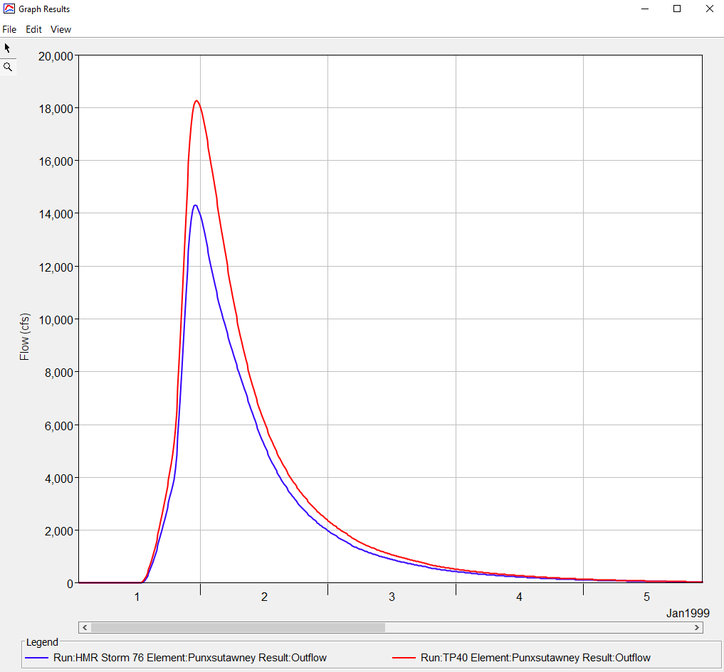
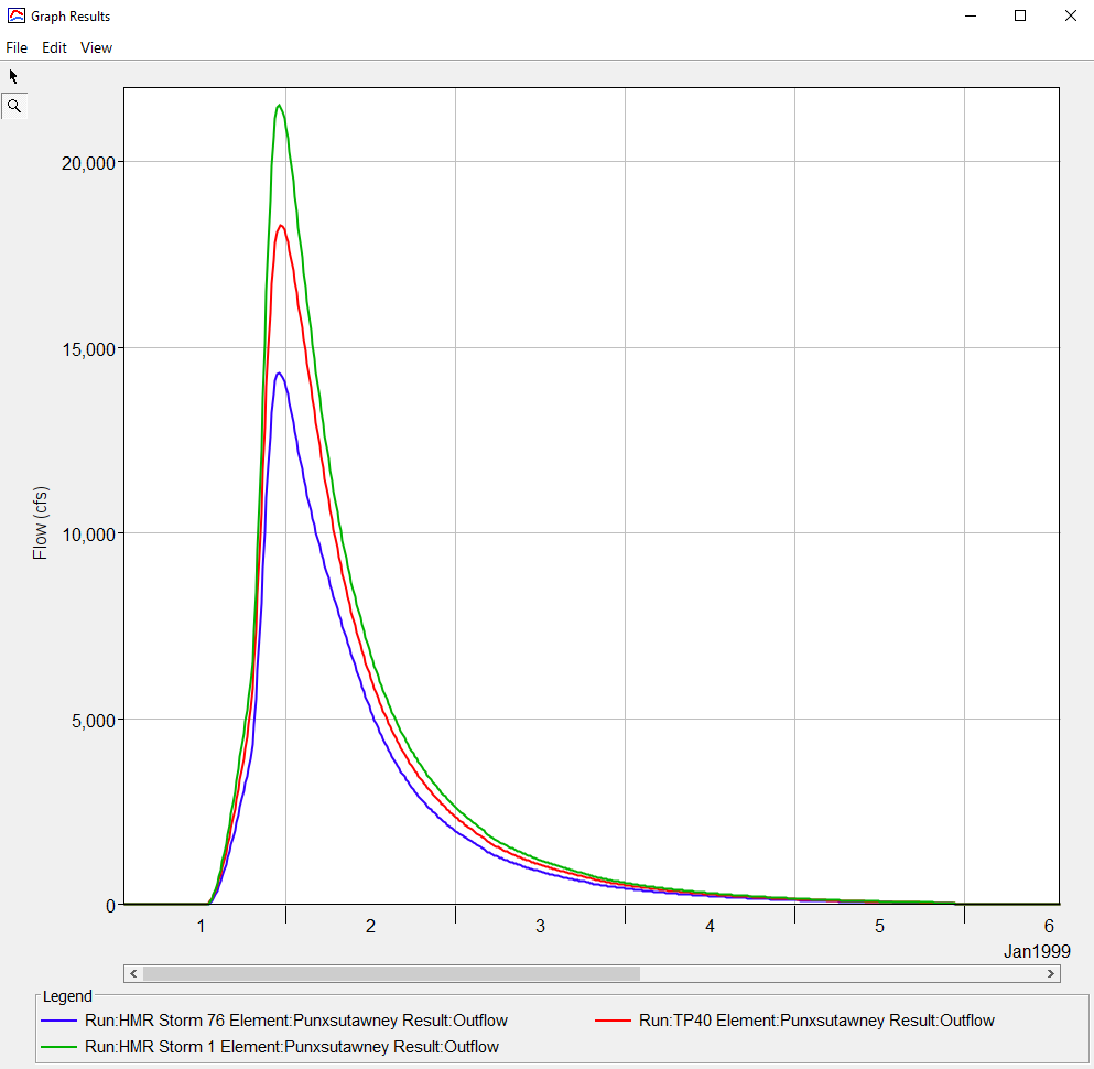
3. Plot the Punxsutawney Outflow hydrograph from both simulations on the same plot. 

Question 1: What is the difference in peak discharge at the Punxsutawney outlet for the two simulations? What is the difference in volume? Were these results expected? Why or why not?

Question 2: How could using the area-reduction curves from historic Storm 76 affect your model? Is additional storm analysis needed?

6. Extra Task 1: Use Area-Reduction Information from a Second Historic Storm in HMR51

The example used earlier in this workshop produced area-reduction factors that were smaller than the TP40 area-reduction factors. These smaller factors caused decreases in depths, outflow, and volume. Another possibility is a historic storm that contains area-reduction factors that are larger than the factors in TP40. For example, HMR 51 Storm 1 has this effect. An additional Excel sheet has been included in the spreadhseet under the tab Extra Task 1 showing area-reduction curves for Storm 1 in HMR 51.

1. Create a new meteorologic model named HMR Storm 1 (it is probably easiest to copy the HMR Storm 76 model as the only parameters that will change are the area-reduction functions associated with the durations).
2. Create new paired data Area-Reduction Functions called 6hr_ARF_1, 12hr_ARF_1, and 24hr_ARF_1 similar to what was done in Task 4, steps 12-14. This time use the reduction information produced from HMR Storm 1 in the spreadsheet, Extra Task 1 tab.
3. Go to the Watershed Explorer and select Meteorological Models | HMR Storm 1 | Frequency Storm. Associate the newly created area-reduction functions from HMR Storm 1 with the appropriate durations as seen below.
    
4. Create a new simulation, called HMR Storm 1 that references the meteorologic model for Storm 1 that you just created.
5. Run the simulation and compare results from all three 1% simulations (TP40, HMR Storm 76, and HMR Storm 1).

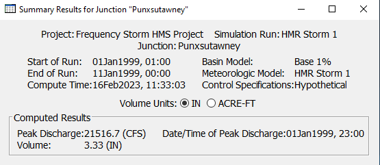
Question 3: What are the differences in peak discharge for each run? What do the two historic storms in HMR51 tell us about the importance of area-reduction information?

7. Extra Task 2: Create a Depth-Area Analysis Simulation

Up to this point in the workshop, a storm area of 158 square miles has been used. This is the drainage area at the most downstream outlet of the model, the Punxsutawney junction element. The computed results at other locations, like the Big Run junction element, do not reflect the correct 1% flow.  To compute the correct 1% flow at the Big Run junction, a storm area of 70 square miles would need to be defined in the meteorologic model which is equivalent to its upstream drainage area. When evaluating multiple points, it could be tedious to create multiple copies of the meteorologic model and then vary the storm area.

The Depth-Area Analysis simulation type includes a built-in capability where the program runs multiple variations of the frequency storm meteorologic model; each variation has a different storm area. HEC-HMS allows the modeler to choose multiple points within the basin model within the depth-area analysis. When computing the analysis, the program will compute the drainage area at each of the defined locations and then use the area and the area-reduction curves to create a storm with the right area-reduction information applied.

Depth-Area Analysis

The Depth-Area Analysis simulation type in HEC-HMS is handy when you are interested in computing a single frequency, such as the 100-yr (1% AEP) flow event, at multiple elements throughout a basin model. The analysis automatically adjusts the storm area for each analysis point based on it's specific upstream drainage area and applies the appropriate area-reduction factor. 

If, instead, you are interested in computing multiple frequencies for only a handful of basin elements, then consider using the Frequency Analysis simulation type in HEC-HMS. After running this simulation type, it automatically creates a flow-frequency (or stage-frequency) curve for the basin element of interest.

1. Create a new depth-area analysis named Depth-Area TP40. Make sure to choose the TP40 meteorologic model.
2. After the depth-area analysis has been created, go to the Compute tab and select the depth-area analysis to open the component editor.
3. Enter a Start Date of 01Jan1999, a Start Time of 01:00, an End Date of 11Jan1999, and an End Time of 00:00. Set the Time Interval to 15 minutes.
4. Select the Analysis Points tab. Select the Punxsutawney junction as Point 1 and the Big Run junction as Point 2 as seen below. 
   
5. Run the depth-area analysis. There are really two simulations that happen during the compute. For Point 1, HEC-HMS will apply area-reduction factors for a storm area of 158 square miles and run the entire basin model.  For Point 2, HEC-HMS will apply area-reduction factors for a storm area of 70 square miles and run the basin model to the Big Run junction. 
6. Results for the depth-area analysis should be viewed from the Results tab of the Watershed Explorer, as shown in the below figure. The Peak Flow Summary Table contains the correct “area-reduced” results for each analysis point. Below the summary table, there is a separate folder with results for each of the analysis points.  Notice the folder only contains results for the elements upstream of the analysis point. 
   

Question 4: Which results from the depth-area analysis would you use for a steady flow HEC-RAS model? Which results from the depth-area analysis would you use for an unsteady flow, 1D HEC-RAS model? Assume that the HEC-RAS model extents are from the Big Run junction to the Punxsutawney junction.

Project Files

Download the final project files here:

Frequency_Storm_HMS_Project_Final.zip