Download PDF
Download page Creating Depth-Area Reduction Curves from Gridded Precipitation Data.
Creating Depth-Area Reduction Curves from Gridded Precipitation Data
Software Version
HEC-MetVue version 3.1 was used to create this tutorial. This software can be downloaded here: https://www.hec.usace.army.mil/software/hec-metvue/downloads.aspx. A version of Microsoft Excel, or other spreadsheet software, will also be required.
Suggested Time
This tutorial should take approximately 30-minutes to complete.
Background
Frequency based precipitation information is often available for point, or precipitation gage, locations. When applying point precipitation to a watershed, depth-area reduction (DAR) factors are required to reduce the point precipitation to an average depth that occurs over the watershed. The general pattern observed from historic storms is that the rainfall magnitude decreases as storm area increases. Therefore, depth-area reduction curves are a required component to account for the storm, or watershed, area.
HEC-HMS can automatically apply an area-reduction factor based on the storm area entered into either the Frequency Storm or Hypothetical Storm meteorologic models. However, the area-reduction curves that are hardcoded into HEC-HMS are from Technical Paper No. 40 and may not be accurate for watersheds larger than 400 square miles. The TP40 reduction curves were developed using only drainage areas of 400 square miles or less so the curves flat line and use similar reduction factors for storm area over 400 square miles. Logically, we know that as storm areas increase in size, the reduction factor should continue to decrease. Also, there is evidence that area-reduction varies across the country. For this reason, a new User-Specified option exists in HEC-HMS where modelers can create and specify their own area-reduction curves specific to their area of interest.
In this tutorial and guide, you will learn how to create site specific area-reduction curves from observed gridded precipitation data. By applying site specific area-reduction factors to your flow frequency studies, you can improve the accuracy of the area-reduced rainfall depths for your local watershed.
Goals
In this tutorial and guide, you will:
- Know how to find gridded precipitation datasets and the tools that are available in HEC-HMS to process them.
- Compute Depth-Area Duration (DAD) tables from observed gridded precipitation data.
- Create site specific Depth-Area Reduction (DAR) curves from the DAD table data.
Data
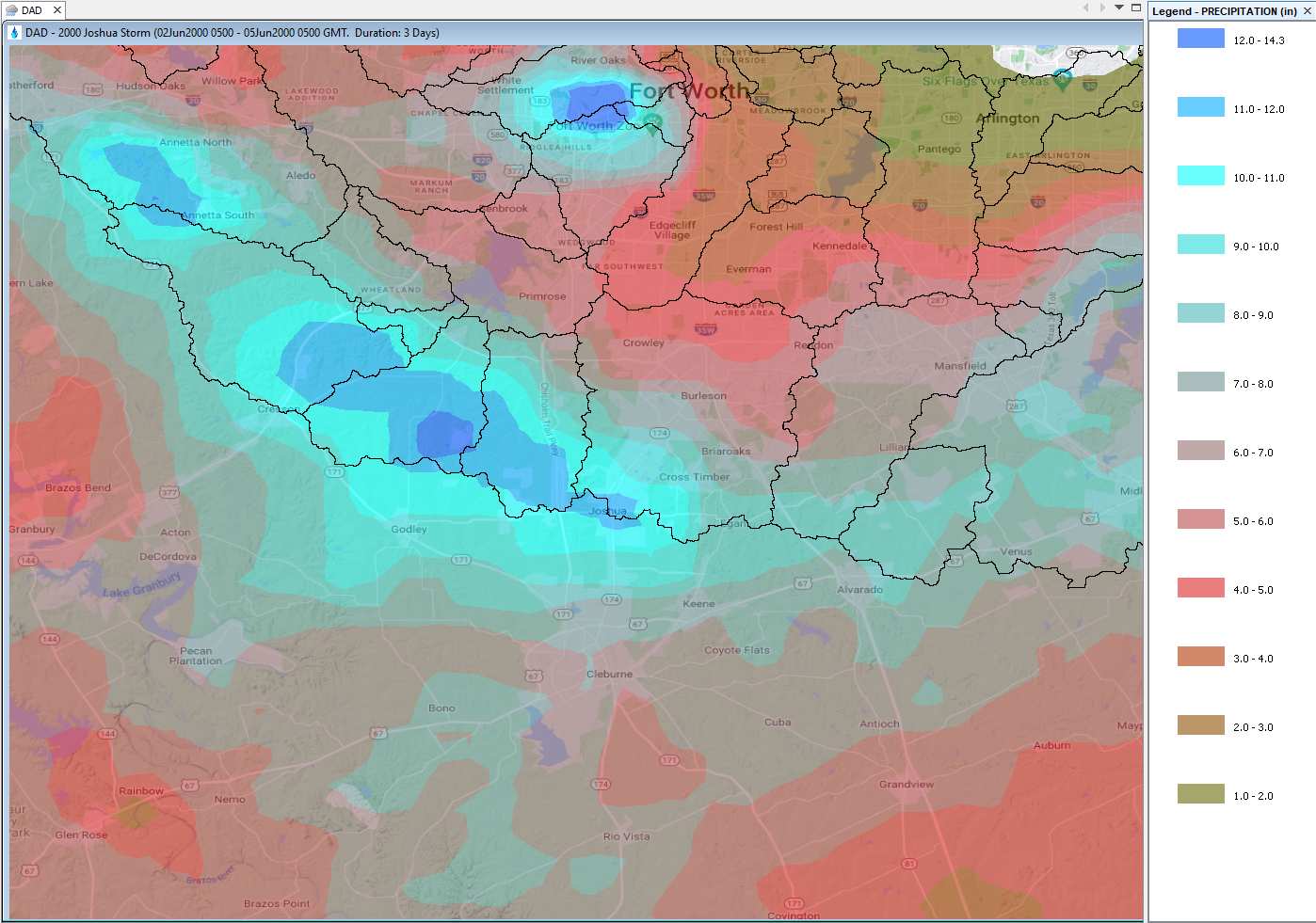
You will be creating DAR curves from a historical event that occurred near Joshua, Texas in early June of 2000. Approximately 14 inches of precipitation fell over the span of three days. Joshua, Texas is located just south of Fort Worth and is partially within the Upper Trinity River watershed.
1. Gather Observed Gridded Precipitation Data
As part of this tutorial and guide, QPE precipitation data for the Joshua event has been retrieved from the West Gulf River Forecasting Center and is provided to you in HEC-DSS file format. For a list of commonly used precipitation gridded datasets, please see the Gridded Data Sources link. For creating depth-area reduction curves, hourly and sub-hourly datasets are recommended. These datasets often come in different file formats such as GRIB or NetCDF. New gridded data tools in HEC-HMS or in standalone Vortex are available to quickly import these datasets into HEC-DSS file format and include options to clip, resample, and reproject the data. Be sure to check out the tutorials and guides relating to using Vortex stand-alone or HEC-HMS for helpful hints and examples of how to manipulate many of these precipitation datasets.
2. Add and Visualize Precipitation Data with HEC-MetVue
- Open HEC-MetVue.
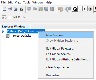
- In the Explorer Window, create a session by right-clicking on the Project File line. Select New Session. Name the session DAD.
- For viewing purpose, let's add a map file of the Upper Trinity River watershed. Expand the nodes under the DAD session node until you see the map data node. Right-click and then select Select Maps.
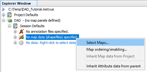
- Click Add Maps and then navigate to and select the Upper Trinity River subbasins shapefile from the initial files download. Click OK.
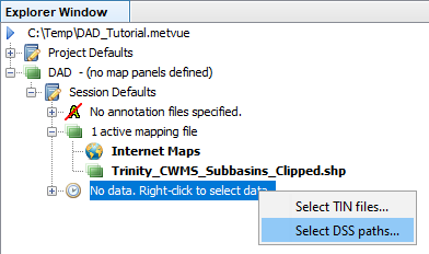
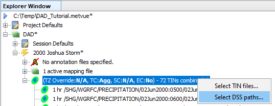
- Now let's add precipitation data. Notice the node labeled No data. Right-click to select data. Right-click that node and then select Select DSS paths.
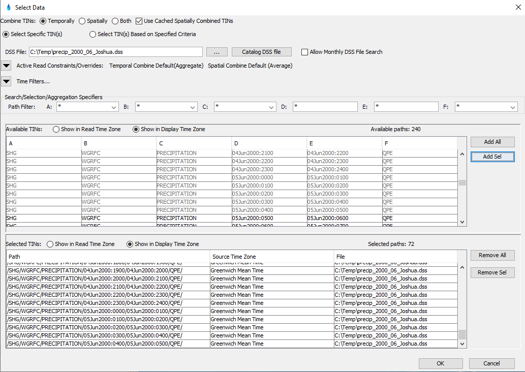
- On the Select Data pane that opens, click the ellipses button (...) to select your DSS file for the 2000 Joshua storm. The DSS file contains about 10 days of precipitation data, but the majority of the rainfall fell during the 72 hours beginning on 02Jun2000:0500 and ending on 05Jun2000:0500. Select the 72 grids spanning the time interval and then select the Add Sel button to add the selected grids to the bottom panel as seen below. Click OK.
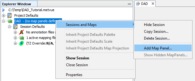
- Now that we have added the necessary data to our DAD session, we need to create a Map Panel to actually interact and work with the data. Right-click the DAD session node then select Sessions and Maps and then select Add Map Panel. Name the map panel 2000 Joshua Storm.

HEC-MetVue Terminology
A Session is a grouping of Map Panels. Sessions are used to organize Map Panels that contain related datasets such as precipitation files. Map Panels have to be created to actually work with the datasets.
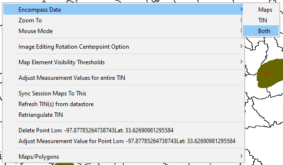
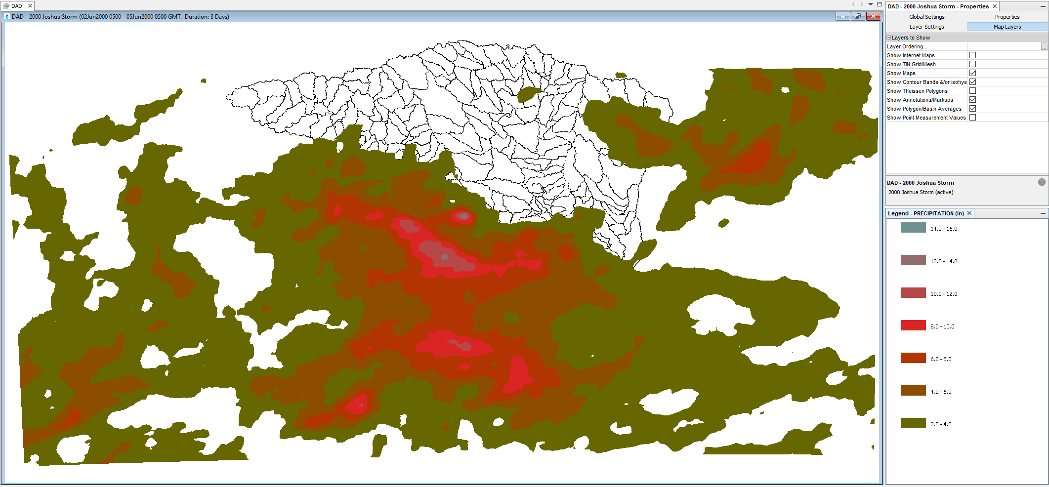
- You should now be able to visualize the Upper Trinity subbasin shapefile and accumulations of the precipitation data you added in the map panel window. To view the entire dataset, right-click in the map panel window and select Encompass Data then Both.
- Steps 9 through 13 are OPTIONAL and should NOT be completed for this specific tutorial and guide. The next few steps are for illustration purposes only to show how to clip storm data in HEC-MetVue if needed. Sometimes when working with gridded precipitation, the spatial extent of the data can be extremely large spanning over multiple states and entire regions of the country. If this is the case, there is a tool in HEC-MetVue that can be used to clip the precipitation data to the area of interest. With the Joshua storm data, the precipitation has already been clipped and no further refinement is necessary.
- Along the top menu bar, select the button below that is highlighted in red. This button allows the user to select a subset of the available storm data.

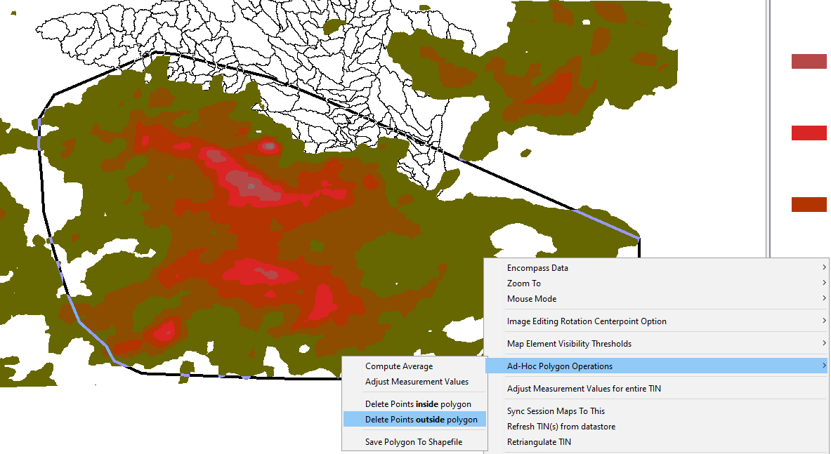
- Next, left-click around the portion of the storm data that you would like to include in the DAD analysis. This will form a polygon. When the polygon is complete, right-click anywhere in the map panel and select Ad-Hoc Polygon Operations then Delete Points outside polygon.
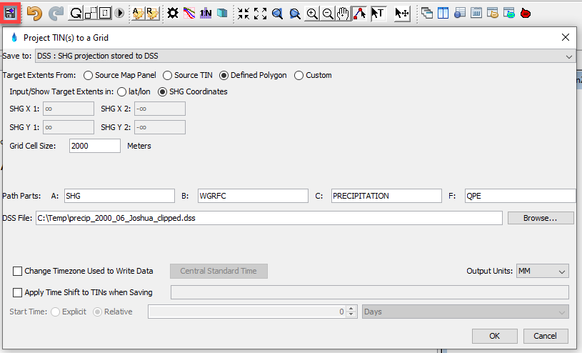
- If the goal is to compute the DAD tables based on the clipped data, the data will need to be saved. Clicking the button below that is highlighted in red and filling out the subsequent save window that pops up will save the clipped data to a new DSS file.
- Even though the clipped data is what is now visible in the map panel, the original, unclipped base data is what HEC-Met-Vue would currently use to compute DAD tables. To use the clipped data, right-click on the data node in the Explorer Window and select Select DSS paths. Then point to the new DSS file where the clipped data is stored.
3. Compute Depth-area Duration Tables with HEC-MetVue
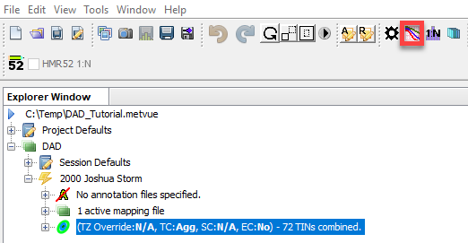
- Within the Explorer Window, make sure that the precipitation data on which you wish to perform a DAD analysis are selected. Then select the DAD button located on the top tool bar.
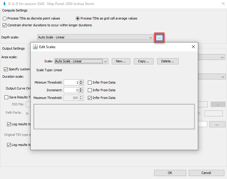
- For Depth Scale, choose Auto Scale - Linear and then select the ellipses (...) button. Set the scale setting according to the below figure.
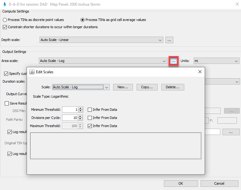
- For Area Scale, choose Auto Scale - Log and then select the ellipses (...) button. Set the scale setting according to the below figure.
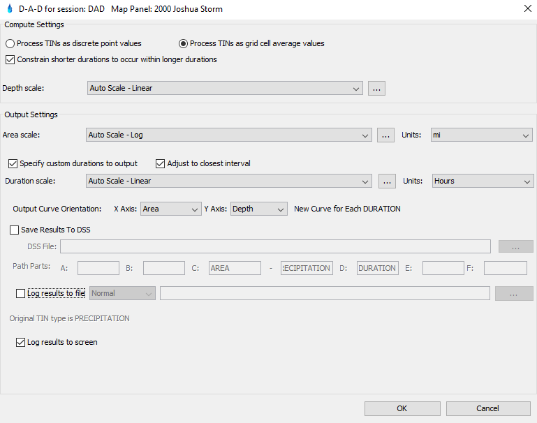
- The DAD panel settings and inputs should now reflect the selections seen below. Click OK to compute the DAD table for the Joshua storm event. Results will be logged to the Output panel screen. Alternatively, you can save results to a text file.
4. Create Depth-area Reduction Curves in Excel
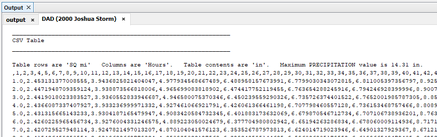
- Within the HEC-MetVue Output panel screen and the DAD (2000 Joshua Storm) tab (seen in the figure above), click anywhere. Press CTRL+A to select the entire table, then press CTRL+C to copy the entire table.
- Open the area_reduction_curves.xlsx file in Microsoft Excel. In the first tab, labeled 2000.06_DAD, click in cell A1 and then press CTRL+V to paste the table copied from HEC-MetVue.
- The text is comma-separated. Within Mirosoft Excel, select all of Column A. Then in the top toolbar, select Data and then Text to Columns. Proceed through the Convert Text to Columns Wizard that pops up Be sure to choose the Delimited file type and select Comma as the delimeter.
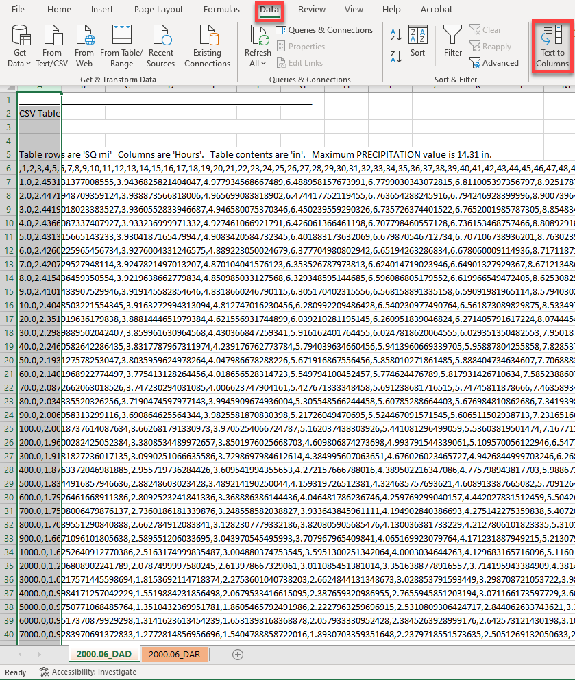
The 2000.06_DAD tab should now appear as below with the decimal depth values starting on column B, row 7.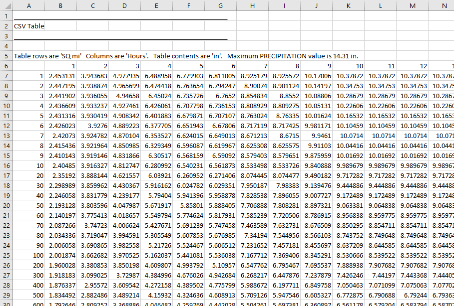
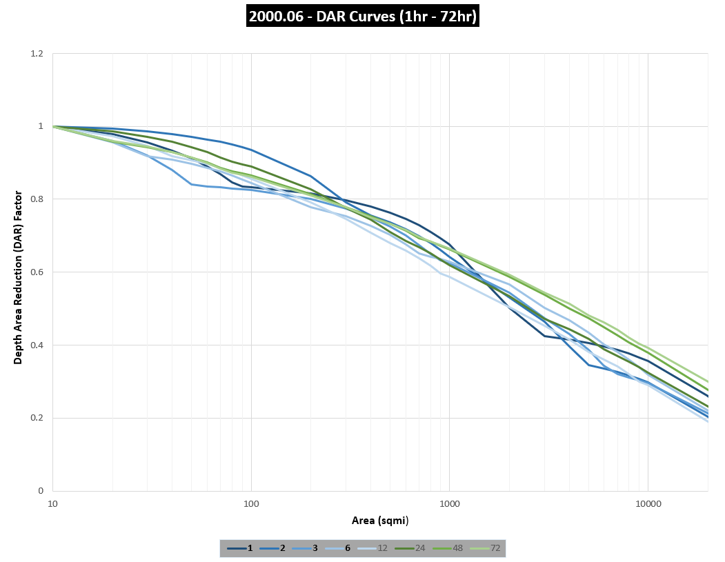
- The pasting and reformatting of the depth-area duration table values in the previous step should automatically generate the depth-area reduction curves on the subsequent tab labeled 2000.06_DAR as seen in the figure below. Notice that the line chart has been automatically configured to only show the "study-friendly" durations that are typically analyzed and found in precipitation-frequency datasets such as those in NOAA Atlas 14. Also, you might have noticed that the DAR factors begin at 1 at the 10 square mile mark. Although not necessary, this is consistent with many historical studies. It can be assumed that precipitation gage data networks are not dense enough to capture the exact storm center peak. Similarly, the spatial resolution of some radar-based precipitation datasets might not be fine enough to capture the storm center peak. So starting the DAR curves at 10 square miles as opposed to 1 square mile can account for this assumption.
Precipitation Frequency Data
Most precipitation-freqruency data, such as that found in NOAA Atlas 14, are point estimates. The data should never be used to generate synthetic storms without applying area-reduction. For example, if the 1/100 annual exceedance probabilty (AEP) for a 24-hour event is 10.0 inches at a point, it is unrealistic to expect that a storm of that same frequency could have ~10.0 inch depths throughout an entire 1,000 square mile watershed. The depths must be reduced as you move away from the storm center and towards the outer storm fringes in order to more closely reflect real, observed storms.
DAR Curves in HEC-HMS
Flow frequency studies are often performed in HEC-HMS by using the Hypothetical Storm or Frequency Storm meteorologic models and assuming that a storm of a certain frequency will lead to a flood event of that same frequency. Both the Hypothetical Storm and Frequency Storm models require point precipitation-frequency data as inputs to build synthetic storms, therefore it is extremely important to adequately reduce the storms using depth-area reduction curves. To see examples of how depth-area reduction curves are applied in these hypothetical meteorologic models, see the tutorials below.
Project Files
Download the final project files here: