Applying the Hypothetical Storm Met Model in HEC-HMS

Software Version

HEC-HMS version 4.11 beta 10 was used to create this tutorial. You will need to use HEC-HMS version 4.11 beta 10, or newer, to open the project files.

Suggested Time

This workshop should take approximately 1-hour to complete.

Project Files

Download the initial project files here:

Village_Creek_HMS_Initial.zip

Goals

In this workshop, you will:

• Create a site-specific temporal storm pattern based on an observed historical storm.
• Apply the Hypothetical Storm meteorological model to estimate frequency flows at a point of interest for the 1/100 annual exceedance probability (AEP).
• Investigate the impact that applied temporal storm patterns have on computed flow results.
• Investigate the difference between the two Spatial Distribution options: 
  • Uniform For All Subbasins.
  • Variable By Subbasin.
• Apply the Ensemble Analysis compute type in HEC-HMS to compare different Simulation Runs.

Data

You will be using an HEC-HMS model of the Village Creek watershed for this workshop. This watershed is located near Beaumont, Texas in the southeastern portion of the state and is approximately 1,130 square miles. A location map and an image of the HEC-HMS basin model configuration can be seen below.

1. Gather Precipitation Frequency Depth-Duration Data from NOAA Atlas 14

NOAA Atlas 14 provides point precipitation frequency estimates. Unlike the Frequency Storm meteorologic model which needs depth estimates for multiple durations due to its balanced hyetograph approach, the Hypothetical Storm method only needs one depth grid that reflects the frequency and total duration of the desired synthetic storm. In this workshop, we are interested in the 1/100 AEP. For the synthetic storm's duration, we will use a 96-hour duration since several of the large, observed storm events near the Texas Gulf have reflected this behavior.

Storm Duration

There are several schools of thought when it comes to choosing a total storm duration for your synthetic storm event. You typically want to limit yourself to a "friendly" duration based on the available NOAA Atlas 14 datasets (i.e. 6-hr, 12-hr, 24-hr, 48-hr, etc.). One simple approach is to choose the shortest "friendly" duration longer than the time of concentration to your outlet. So if the time of concentration is 20 hours, you may want to choose a storm duration of 24 hours. A second approach would be to choose a duration tied to the meteorology. In this workshop example, many of the historic, tropical storms seen in this region near the Gulf last three to four days so a 96 hour duration was chosen. A third approach would be to determine the critical duration that leads to the most conservative, yet defendable answer. For example, a sensitivity analysis could be done by modeling several synthetic storms each with different durations and then choosing the duration that leads to the "worst" result.

1. Go to NOAA’s Precipitation Frequency Data Server web page (https://hdsc.nws.noaa.gov/hdsc/pfds/) and click on the state of Texas (TX). 
2. Change the Time series type option from Partial Duration to Annual Maximum.
3. Type in “Beaumont, TX, USA” as the location (use option C to define the location by address).
4. The frequency-depth-duration table will populate below the map as shown in the below figure. The values in the table reflect a point precipitation frequency estimate. When modeling storms occurring over a watershed, you want to determine the average "point" precipitation depth. In some watersheds, the point precipitation can vary significantly throughout the watershed. You might only use the point precipitation table if your watershed is less than a few square miles. 
   
5. In this workshop, a 1/100 AEP, 96-hour duration storm will be simulated. HEC-HMS now has the ability to ingest NOAA Atlas 14 precipitation-frequency grids directly and compute the average depth for the entire watershed or for individual subbasins. These grids can be found on the NOAA Atlas 14 website within the Supplementary Information tab as shown below. For this workshop, we are interested in the 1/100 annual exceedance probability and the 4-day duration. This grid has already been downloaded for you and is located in the data folder in your HEC-HMS project directory. Although not needed for the Hypothetical Storm meteorologic model, this project also contains two Frequency Storm meteorologic models which need multiple grids for each duration. So you will notice that grids for other durations are also located in the data folder. 
   
6. For this workshop, the NOAA Atlas 14 precipitation-frequency grids have already been imported into HEC-HMS as seen below. It is important to note, however, that there is now a tool to rapidly import NOAA Atlas 14 precipitation-frequency grids into HEC-HMS. To access the Precipitation Frequency Grid Importer, click File | Import | Gridded Data | Precipitation Frequency. 
   

2. Create Temporal Storm Pattern

Now, we will use a gridded precipitation dataset from a historical event to create an observed time-pattern percentage curve. As seen in the figure below, a time-pattern percentage curve goes from 0 - 100 % on the x-axis (time) and also from 0-100 % on the y-axis (precipitation depth). A time-pattern percentage curve will eventually be applied to our hypothetical storm to dictate how the 1/100 AEP, 96-hour depth is distributed temporally.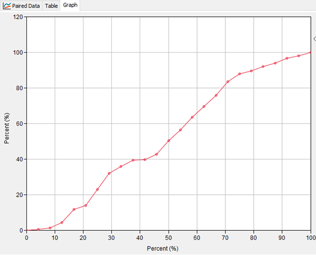

For this workshop, we will use a large storm event observed over the Village Creek watershed in October of 2006. The peak, accumulated depth observed over the ~96-hour storm event falls well within the NOAA Atlas 14 lower and upper confidence limits for the 1/100 AEP, 96-hour point frequency depth for the Village Creek watershed. Thus this is an appropriately large storm event from which to derive a time-pattern percentage curve given the goal of predicting 100-year frequency flows for Village Creek.

1. Gridded precipitation data from the October 2006 event have already been downloaded and processed for you. The processed data can be found in the data folder of your HEC-HMS project directory in the file named 2006_10_Event.dss. The HEC-HMS gridded data importer (found under File | Import | Gridded Data | Importer) was to used to convert the data from their native NetCDF format to DSS and to clip the data with a buffered shapefile of the Village Creek watershed.

   

   Gridded Boundary Condition Data

   For a repository of available gridded datasets for hydrologic boundary conditions such as precipitation, temperature, and snow water equivalent (SWE), see the following link: gridded data sources. For this example, Analysis of Period of Record for Calibration (AORC) gridded precipitation data were downloaded and processed via the HEC-HMS Importer tool. For computational and file storage efficiency, it is recommended to use the Importer tool to clip gridded data so that it only extends a little further than the basin boundary polygon.

2. In order to create a time-pattern percentage curve from the observed October 2006 event, we first need to derive a basin-average, incremental precipitation time-series from the gridded dataset. We will achieve this goal using the Grid to Point tool in HEC-HMS.
3. Open HEC-HMS software. Along the top menu bar, open the Grid to Point tool by navigating to Tools | Data | Grid to Point.
4. For the Source File, navigate to the data folder of your HEC-HMS project directory and choose 2006_10_Event.dss. Select all of the Source Grids and move them to the right pane as seen below. Click Next.
   
5. For the Zones Shapefile input, navigate once again to the data folder and select the shapefile named village_ck_dissolved.shp. For the Field, select name. Click Next.
6. For Select Destination, navigate to the data folder and name the output DSS file 2006_10_GridToPoint as seen below. Click Open.
   
7. Specify names for DSS Parts A and F as seen below. Click Next to generate the basin average time-series. Then click Close and OK to exit the Grid to Point tool. 
   
8. Open the newly created 2006_10_GridToPoint.dss file, select the pathname with PRECIP-INC as the Part C name, and then select the tabulate button. Also, open the time_pattern_percent_curve_initial.xlsx spreadsheet which is part of the initial project files for this workshop.
   

9. Within the DSS file, copy the entire depth column which should consist of about 97 total basin-averaged depths.
   

   

   Data Units

   The unit system for the native precipitation data used in this example is metric. However, there is a view setting in HEC-DSSVue that might automatically convert the data to U.S. units as seen below. Either way, the end result should be the same since the spreadsheet calculates the Time (%) and Cumulative Precip (%) columns based on percentages.
   

10. Next, paste the values from DSS into the time_pattern_percent_curve_initial.xlsx spreadsheet, starting in cell C2. The rest of the spreadsheet should automatically populate for you. 
    
    The completed table above now contains the incremental basin average precipitation for a Village Creek storm event that occurred in October of 2006. The total storm precipitation was about 266.90 millimeters (10.51 inches) over a 96-hour period. The precipitation was normalized by dividing the incremental precipitation values by the storm total. Then, the cumulative percent time and percent normalized precipitation were computed as shown in the highlighted columns. The percent time column was computed by dividing the current duration by the total storm duration; the total storm duration was 96 hours in this example. When defining a temporal pattern percentage curve in HEC-HMS, both independent (percent storm duration) and dependent (percent total depth) variables must start at 0 percent and end at 100 percent.
11. In the next section of this workshop, we will use the highlighted columns to build a time-pattern percentage curve in HEC-HMS.

3. Apply the Hypothetical Storm Meteorologic Model

Now that we have all the necessary data, we will apply the Hypothetical Storm meteorologic model to estimate frequency flows at a point of interest for the 1/100 annual exceedance probability (AEP). 

1. Open the HEC-HMS project named Village_Creek.hms in the downloaded workshop folder. Some context to the initial project setup is provided below.
   • A basin model has been created for you and is calibrated to model large flood events.
   • Two Frequency Storm meteorologic models have been created for you, along with two Simulation Runs. The results from these runs will be used later on in this workshop to compare/contrast with the Hypothetical Storm meteorologic models that you will create and run.
   • A generic Control Specification that spans 8 days has been created for you.
   • Under Paired Data, 18 Percentage Curves have been created for you based on temporal data downloaded from NOAA Atlas 14.
   • Under Paired Data, nine Area-Reduction Functions have been created for you based on large historical storms observed near the Village Creek watershed. Although all nine are needed for the Frequency Storm meteorologic models, only one (the 96hr_100yr curve) is needed for the Hypothetical Storm meteorologic models you will create.
   • Under Grid Data, nine Precipitation-Frequency Grids have been imported using the Precipitation Frequency Grid Importer. Although all nine are needed for the Frequency Storm meteorologic models, only one (the tx100yr04da_ams grid) is needed for the Hypothetical Storm meteorologic models you will create.
2. Create a new meteorologic model.
3. Enter the name Hypo Storm Uniform Oct 2006 and click Create.
4. In the Watershed Explorer, select the new meteorologic model you just created to open the component editor.
5. Change the Precipitation option to Hypothetical Storm. Make sure the Unit System is set to U.S. Customary.
6. Click the Basins tab. Change the Include Subbasins option from No to Yes for the Village_Creek basin model.
7. Now click on Hypothetical Storm under your Hypo Storm Uniform Oct 2006 meteorologic model.
8. For Method, change the selection from Area-Dependent Pattern to User-Specified Pattern.
9. Skip the Storm Pattern selection for now. Move ahead to the Storm Duration (HR) option and enter 96.
10. Change the Precipitation Method option from Point Depth to Precipitation-Frequency Grid. For Grid, select the tx100yr04da_ams grid.
11. For Computation Point, select Basin: Village_Creek, Element: NechesRv_Nr_Beaumont.
12. For the Area Reduction option, change the selection to User-Specified, then choose the 96hr_100yr area reduction function.
13. The selected computation point, NechesRv_Nr_Beaumont, has a total drainage area of 1130.1 square miles. You do not have to enter a storm area. HEC-HMS will use the drainage area of the selected computation point if no storm area is defined. You would enter a storm area if you want to override the computation point's drainage area. 
14. For Spatial Distribution, select Uniform For All Subbasins. 
15. Click Save. The Frequency Storm component editor should now look identical to the below figure.
    
16. The last step to completing this Hypothetical Storm met model is to set the Storm Pattern parameter to reflect the temporal pattern observed in the October 2006 historic event; first we have to create the Percentage Curve in HEC-HMS using the highlighted columns from the time_pattern_percent_curve_initial.xlsx spreadsheet.
17. Go to Components | Paired Data Manager. Change the Data Type to Percentage Curves and click New. Name the curve Oct_2006_Event_96hr and select Create.
18. In the Watershed Explorer, expand the Paired Data folder, then expand the Percentage Curves folder, and select Oct_2006_Event_96hr. 
19. In the Component Editor below, click the Table tab. From the spreadsheet, copy the highlighted Time (%) column values (D2:D98) and then paste them into the left table column in HEC-HMS. Copy the highlighted Cumulative Precip (%) column values (F2:F98) and then paste them into the right table column in HEC-HMS.
20. Now click on the Graph tab. Your Percentage Curve should like the below figure.
    
21. Now navigate back to the Hypo Storm Uniform Oct 2006 met model and select Hypothetical Storm. For the Storm Pattern option, select the Oct_2006_Event_96hr percentage curve that you just created.
22. Lastly, create a Simulation Run to compute the hypothetical storm. Go to Compute | Simulation Run Manager and select New.
23. Name it after the met model, Hypo Storm Uniform Oct 2006 and click Next. Select the Village_Creek basin model and click Next. Select the Hypo Storm Uniform Oct 2006 met model and click Next. Now select the Simulation Window Control Specification and then click Finish. 
24. Run the Hypo Storm Uniform Oct 2006 simulation. Under the Results tab, expand this simulation run node and look at the Graph and Summary Table for NechesRv_Nr_Beaumont. 

Question 1: What is the peak discharge (estimated 1/100 AEP) for the NechesRv_Nr_Beaumont outlet? How many distinct hydrograph peaks can be observed at the NechesRv_Nr_Beaumont outlet? Given the percentage curve derived from the observed October 2006 storm event, does this surprise you?

4. Investigate the Impact of the Two Spatial Distribution Options

The Hypothetical Storm automates the process of calculating average precipitation-frequency depths for the entire watershed or for individual subbasins. HEC-HMS offers two options for calculating average precipitation-frequency depths, Uniform For All Subbasins and Variable By Subbasin. The uniform option generates a bounding polygon that includes all subbasins above a user-defined computation point. The program will intersect the precipitation-frequency grid with the bounding polygon to calculate the area average precipitation-frequency depth. So, when using the uniform option, all subbasins upstream of a computation point will receive the same rainfall hyetograph. For watersheds with higher precipitation variability among individual subbasins, the variable by subbasin option can be used to apply average point precipitation-frequency values for each individual subbasin. Both options will be investigated in this section of the workshop.

1. Create a copy of the Hypo Storm Uniform Oct 2006 meteorologic model and name it Hypo Storm Variable Oct 2006.
2. Open the Hypothetical Storm Component Editor in the Hypo Storm Variable Oct 2006 meteorologic model. As shown below, change the Spatial Distribution option to Variable By Subbasin.
    
3. Create a copy of the Hypo Storm Uniform Oct 2006 simulation and name it after the newly created met model, Hypo Storm Variable Oct 2006. The only thing that will change from the copied simulation is the associated met model; make sure you select the correct meteorologic model within the new Hypo Storm Variable Oct 2006 simulation as shown below.
   
   
4. Run the Hypo Storm Variable Oct 2006 simulation. You should notice the following messages in the message log console. You can see the subbasin average precipitation depth values and the values after the precipitation was reduced for a storm area of 1130.1 square miles. The program automatically computed the subbasin average depth values using GIS operations and the precipitation-frequency raster and subbasin polygons.
   NOTE 23413:  Area upstream of computation point: 1,130.15 MI2.
   NOTE 23407:  Hypothetical storm area: 1,130.1 MI2.
   NOTE 23414:  Hypothetical storm depth for subbasin VillageCk _S10: 19.111 IN.
   NOTE 23409:  Area-reduced hypothetical storm depth: 13.772 in.
   NOTE 23414:  Hypothetical storm depth for subbasin VillageCk_S20: 18.742 IN.
   NOTE 23409:  Area-reduced hypothetical storm depth: 13.506 in.
   NOTE 23414:  Hypothetical storm depth for subbasin VillageCk_S30: 22.029 IN.
   NOTE 23409:  Area-reduced hypothetical storm depth: 15.875 in.
   NOTE 23414:  Hypothetical storm depth for subbasin Neches_S150: 22.84 IN.
   NOTE 23409:  Area-reduced hypothetical storm depth: 16.459 in.
   

5. Now, let's quickly re-run the Hypo Storm Uniform Oct 2006 simulation and analyze the message output when the Spatial Distribution option is uniform. In this case, the computation point is set as the NechesRv_Nr_Beaumont element which is located at the outlet of the basin model. So when calculating the hypothetical storm depth, the precipitation-frequency grid is intersected over the entire basin polygon, leading to a single basin-average depth value of 19.671 inches that is applied uniformly to each subbasin. As you can see below, the same area-reduced depth is applied to each subbasin. 
   NOTE 23413:  Area upstream of computation point: 1,130.15 MI2.
   NOTE 23407:  Hypothetical storm area: 1,130.1 MI2.
   NOTE 23414:  Hypothetical storm depth for subbasin VillageCk _S10: 19.671 IN.
   NOTE 23409:  Area-reduced hypothetical storm depth: 14.176 in.
   NOTE 23414:  Hypothetical storm depth for subbasin VillageCk_S20: 19.671 IN.
   NOTE 23409:  Area-reduced hypothetical storm depth: 14.176 in.
   NOTE 23414:  Hypothetical storm depth for subbasin VillageCk_S30: 19.671 IN.
   NOTE 23409:  Area-reduced hypothetical storm depth: 14.176 in.
   NOTE 23414:  Hypothetical storm depth for subbasin Neches_S150: 19.671 IN.
   NOTE 23409:  Area-reduced hypothetical storm depth: 14.176 in.
   
   Question 2: For the uniform simulation above, what area-reduction factor was applied? Is the application of an area-reduction factor necessary in this case?
   

   Click for answer...

   The applied area-reduction factor was approximately 0.721 (14.176 / 19.671 = 0.721). The 0.721 reduction factor was determined from the 96hr_100yr area-reduction curve associated with this met model and from the hypothetical storm area of 1,130.1 square miles. 
   
   
   

   The application of an area-reduction factor IS absolutely necessary. NOAA Atlas 14 precipitation-frequency grids provide point depth estimates only. When converting from point depths to an areal depth used in creating synthetic storms, area-reduction must be applied or else a gross overestimation of rainfall will occur. This follows the paradigm that is observed in historical storms which usually have one (or more) intense rainfall centers that lessen in severity as you extend towards the outer fringes of the storm. The only time area-reduction should not be applied in HEC-HMS is if the entered depth value has already been reduced outside of HEC-HMS.
   

   Question 3: Would the application of TP40 area-reduction curves be applicable given this model? Why or why not?
   

   Click for answer...

   No, TP40 area-reduction curves should not be applied to the Village Creek model. As their name implies, TP40 curves were published by the National Weather Service in Technical Paper 40. The rainfall frequency analysis performed as a part of this study was only intended to be applied to catchment areas up to 400 square miles. If extended beyond 400 square miles, essentially no further reduction would result using these curves. The Village Creek watershed is approximately 1,130 square miles. If the TP40 curves were applied to this watershed, the computed rainfall and flow results would likely be overestimated. 
    

6. View the subbasin hyetographs and summary results for the Hypo Storm Variable Oct 2006 simulation at each of the four subbasin elements. As shown below, you should see different hyetographs for all four subbasins. Also, the subbasin results show that all four subbasins have a different total storm depth, matching those values in step 4 above.
   
   

7. If you were to compare results from the uniform precipitation and variable precipitation hypothetical storm simulations at the NechesRv_Nr_Beaumont element, you will see very similar results (less than 1 percent difference). However, you will see larger differences in results at the outlet of individual subbasins. Differences in results become smaller as you work your way downstream because the drainage area approaches the storm area used to reduce the point precipitation depths.  

   

   Uniform vs Variable Spatial Distribution

   In many cases, the Uniform By Subbasin option is a sufficient method of distributing depths spatially over a basin model. The Variable By Subbasin option, however, should be used when the NOAA Atlas 14 depth values vary significantly over the modeling domain. The Village Creek watershed is located near Beaumont, Texas which is roughly 40 miles from the Gulf of Mexico. This region of Texas marks a transition from predominantly convective storm types to larger tropical storms. As a result, the depth gradient changes quickly in this area as demonstrated in the below figure. In this case, the uniform rainfall assumption might lead to the application of too much rainfall in the northernmost subbasins and not enough in the southernmost subbasins closer to the Gulf. 

   

5. Investigate the Impact of Applying Different Temporal Storm Patterns

As seen with the percentage curve derived from the historical October 2006 event, the applied percentage curve associated with the Hypothetical Storm met model can have a significant impact on the timing of the computed flow results. Now we will investigate how the applied percentage curve might affect the computed peak flow result. In this section of the workshop, we will apply different hypothetical temporal patterns derived from NOAA Atlas 14 data.

1. Go to https://hdsc.nws.noaa.gov/hdsc/pfds/pfds_temporal.html.  
2. For this Village Creek project, we are interested in Volume 11, temporal distribution area '3', at a duration of 96-hour.
   
3. For convenience, the appropriate temporal distributions have already been downloaded for you. They are located in the data folder of your HEC-HMS project directory in a file named tx_3_96h_temporal.csv.

4. Open the tx_3_96h_temporal.csv file to look at the data.

   

   NOAA Atlas 14 Temporal Patterns

   There are many different NOAA Atlas 14 temporal patterns to choose from when building a synthetic storm. The patterns in this workshop are from volume 11, temporal distribution area 3 (eastern Texas) and have a total duration of 96-hours which makes them site specific for the Village Creek watershed. The patterns are categorized into quartiles, each of which refers to the quarter of the storm that has the most rainfall depth. Within each quartile, the patterns are further categorized into 9 different percent of occurrence columns (90%, 80%, 70% etc.). The percentile refers to the range of uncertainty for a given quartile. So for the NA14_Q3_50%_96hr curve, the majority of the precipitation falls in the third quartile with the cumulative percentage of total precipitation having occurred by the given time in 50% of cases observed.
   

5. For convenience, paired data Percentage Curves have already been created in HEC-HMS for all of the first and third quartile cases. When creating paired data object in HEC-HMS, the table values are automatically stored in the project DSS file.

6. To plot the curves on the same plot, open the Village_Creek.dss file located in the project directory. Filter the pathnames by toggling the C-Part dropdown to PERCENT GRAPH. Select all of the Q1 entries and then click the plot button.
   
   
   As expected, the majority of the precipitation volume for each curve is applied during the first 25% of the storm duration, which in this case is day 1 of 4. 
   Question 4: Which one of the first quartile curves would you expect might lead to the greatest peak flow estimate at the Village Creek outlet?

   Click for answer...

   Generally, the steepest percentile curves will lead to the largest peak flow estimates. For this example, the 10% percentile curve is the steepest.

   Question 5: Assuming a total storm depth of 10 inches which of the first quartile curves satisfies the following statement: the accumulated amount of rainfall at the halfway mark of the storm (48 hours) is 6.0 inches. 

   Click for answer...

   The NA14_Q1_90%_96hr curves satisfies the statement.
   

   Of all the observed first quartile cases in the eastern Texas study area, 90% of them had at least 60% of their total storm volume in the first 48 hours.

7. Investigate the impact that the choice of a temporal Percentage Curve can have on the computed results. Copy the Hypo Storm Variable Oct 2006 meteorologic model and name it Hypo Storm Variable Q1P90.
8. In the watershed explorer, expand the newly created Hypo Storm Variable Q1P90 met model and change the Storm Pattern option to the NA14_Q1_90%_96hr percentage curve.
   
9. Copy the Hypo Storm Variable Oct 2006 simulation run and name it after the met model, Hypo Storm Variable Q1P90. Be sure to associate the new met model to the new simulation run.
   

10. Run the Hypo Storm Variable Q1P90 simulation and review the results.
    Question 6: How do the outflow results at NechesRv_Nr_Beaumont compare between the Hypo Storm Variable Q1P90 and the Hypo Storm Variable Oct 2006 simulations?

    Click for answer...

    The peak outflow result using the NA 14 temporal curve is about 40,000 cfs lower than the peak outflow result using the historic temporal curve from the October 2006 event.

    

11. Between the remaining 17 NOAA Atlas 14 percentage curves, choose two that you think might lead to the highest peak flow estimates at NechesRv_Nr_Beaumont. Repeat steps 7 - 10 above to create two additional meteorologic models with your chosen percentage curves and two additional simulation runs.

12. Run the two new simulation runs and compare your results.
    Question 7: Which of your simulation runs led to the highest peak flow results?

    Click here for answer...

    Answers will vary. For this solution, the first quartile 10th percentile curve and the third quartile 90th percentile curve were chosen for the two new simulation runs. The first quartile 10th percentile curve led to the highest peak flow estimates.
    
    

    

Selecting a Percentage Curve for a Hypothetical Storm

Hopefully this section of the workshop demonstrated the significant impact that a temporal pattern can have on the computed results. In terms of applying the most suitable NOAA Atlas 14 percentage curve, a good rule of thumb is to choose the quartile that best reflects the large, historic storms that have been observed near the watershed. Once the quartile is chosen, it might be prudent to choose the steepest percentile curve. Applying a temporal pattern derived from an appropriate historic storm is a valid option too. In all cases, performing a sensitivity analysis before settling on a single temporal pattern is highly recommended. Another option is to use multiple temporal patterns and incorporate additional uncertainty into the flow frequency estimate as shown here - https://www.hec.usace.army.mil/confluence/sspdocs/ssptutorialsguides/combining-precipitation-frequency-and-flow-frequency-results/combining-flow-frequency-curves-determined-by-independent-estimates. 

6. Extra Task: Apply the Ensemble Analysis Compute Type to Compare and Aggregate Results

Ensemble modeling is a process whereby multiple base models are created and simulated in a collective fashion to predict an outcome. Each base model may include different basin configurations, modeling methods, parameter sets, initial conditions, and/or boundary conditions. As long as the base models are diverse and independent, the prediction error of the base models decrease when the ensemble modeling approach is used. While the ensemble model is composed of multiple models, it acts and performs as a single model.

1. Create an ensemble analysis using several of the base models (or simulations) that we have already created.
2. From the top menu bar, select Compute | Ensemble Analysis Manager.
   
3. Select New and name the analysis Ensemble_100yrEstimate. Select Simulation Run as the analysis type and then select Next. 
4. All of the simulation runs that have been previously created are available for selecting as part of this ensemble analysis. You can select them by moving them from the left window pane to the right window pane. Choose the Frequency Storm Variable, Hypo Storm Variable Q1P10 and Hypo Storm Variable Q3P90 simulations. Select Next and then Finish.
   

5. Now that the ensemble analysis has been created, we can select and further refine it by selecting the Compute tab of the Watershed Explorer and then selecting the newly created ensemble analysis. 

6. To select the time-series results output that you wish to generate during a compute, select the output gear icon. 
   
   For this analysis, save the cumulative precipitation time-series results for VillageCk_S10. Select the box next to this time-series and then click Save.
   
   
7. Compute the ensemble analysis and view the plot of the cumulative precipitation results for VillageCk_S10. The plot contains traces from each of the three simulation "base models" that make up the ensemble analysis. The plot also contains aggregated statistical time-series, such as the mean cumulative precipitation. While this is a trivial example to demonstrate how to create an ensemble analysis in HEC-HMS (you would need many more ensemble members to determine adequate results), if applied strategically, the aggregated results from an ensemble analysis can often times outperform the result derived from a single base model.
   
   
   

Project Files

Download the final project files here:

Village_Creek_HMS_Final.zip