Combining Flow Frequency Curves Determined by Independent Estimates

Software Version

HEC-HMS version 4.10 was used to create this example. You can open the example project with HEC-HMS 4.10 or a newer version.

Example Files

Example project files can be found here:

HEC-HMS Project - SanLorenzo.zip

Introduction

Bulletin 17C contains guidance for combining independent flow frequency curves. Specifically, Appendix 9 provides an example where information from a Bulletin 17C analysis is combined with a flow frequency estimate from a regional analysis. This example shows how to combine a Bulletin 17C flow frequency curve with flow frequency information from precipitation-runoff modeling using HEC-HMS. The same watershed and model from the Modeling Flow-Frequency Relationships using HEC-HMS tutorial was used as the starting point for this example.

This example only includes uncertainty in the hypothetical storm's temporal pattern. Other sources of uncertainty that could have been included are uncertainty in the precipitation depth, depth-area reduction, spatial pattern, initial conditions and hydrologic process parameters. 

Steps

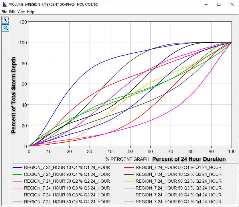
1. Additional temporal patterns were added to the SanLorenzo HEC-HMS project. The Atlas 14 10-, 50-, and 90-percent patterns were added from each quartile. Also, the 2017 time pattern was added; the 1982 time pattern was already in the project. The following figure shows the twelve Atlas 14 temporal patterns that were added to the project (as Percentage Curves). These temporal patterns are saved in the Atlas14TemporalPatterns.dss file located in the ...\SanLorenzo\data directory. 
   
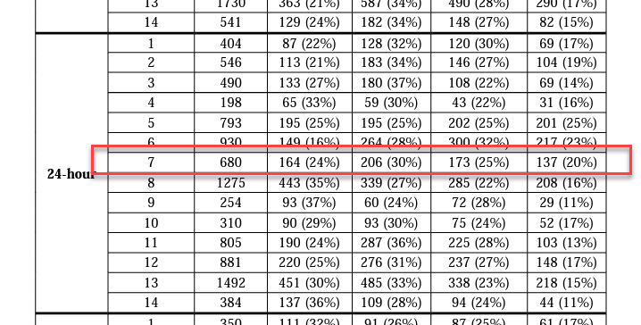
2. The following figure shows a portion of Table A.6.1 in Atlas 14 Volume 6. The San Lorenzo watershed is in California region 7. Table A.6.1 shows 680 storms were used to build the thirty-six 24-hour temporal patterns. Also, the number of events per quartile is somewhat consistent; therefore three time patterns from each quartile were selected. 
   
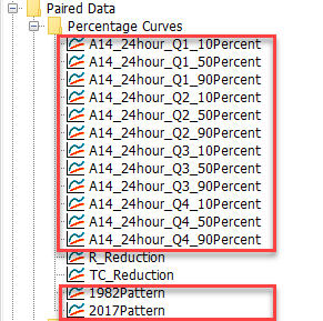
3. The following figure shows all 14 temporal patterns in the HEC-HMS project. 
   
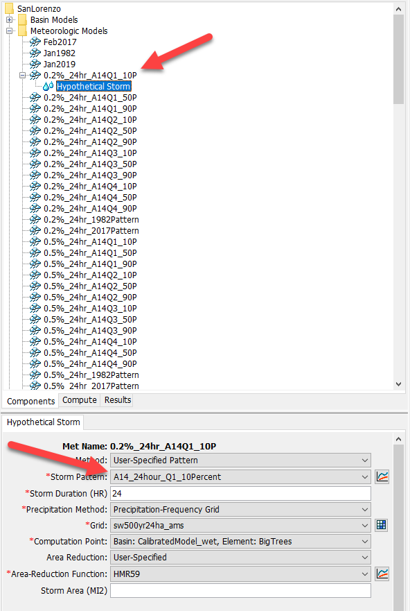
4. A separate meteorologic model was created for each precipitation frequency and temporal pattern combination. There are fourteen temporal patterns, and the example is set up to compute the 50-, 20-, 10-, 4-, 2-, 1-, 0.5-, and 0.2-percent Annual Exceedance Probability (AEP) events. This means 112 separate meteorologic models were added to the project. Descriptive names, based on the temporal pattern, were used to name each meteorologic model. The component editor for each meteorologic model was edited to select the correct temporal pattern. The following figure shows a portion of the meteorologic models and the component editor for the 0.2%_24hr_A14Q1_10P meteorologic model. 
   
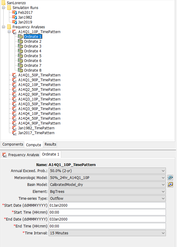
5. The Frequency Analysis compute was a time saver in this example. Instead of creating 112 separate simulation runs, 14 frequency analysis computes were created and configured. The following figure shows all 14 frequency analysis computes, Ordinate 1 in the A14Q1_10P_TimePattern analysis is selected. Ordinate 1 is the 50 percent event, it uses the 50%_24hr_A14Q1_10P meteorologic model. The other seven ordinates have the correct meteorologic models selected (all use the same time pattern). 
   
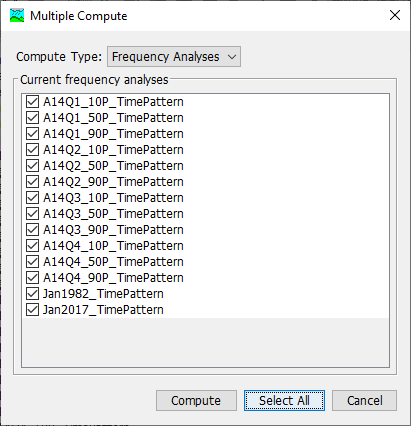
6. The Frequency Analyses were computed using the Multiple Compute option available from the Compute menu. 
   
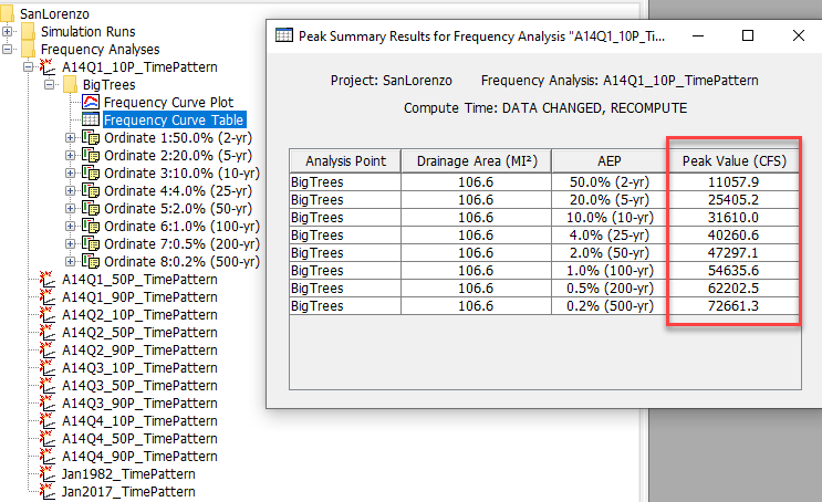
7. Another useful feature of the frequency analysis is that peak flow results at the element of interest are summarized for each ordinate. The figure below shows the flow frequency information for all 8 frequency events using the A14_24hour_Q1_10Percent temporal pattern. 
   

8. The following table contains the flow-frequency results from the HEC-HMS simulations. 

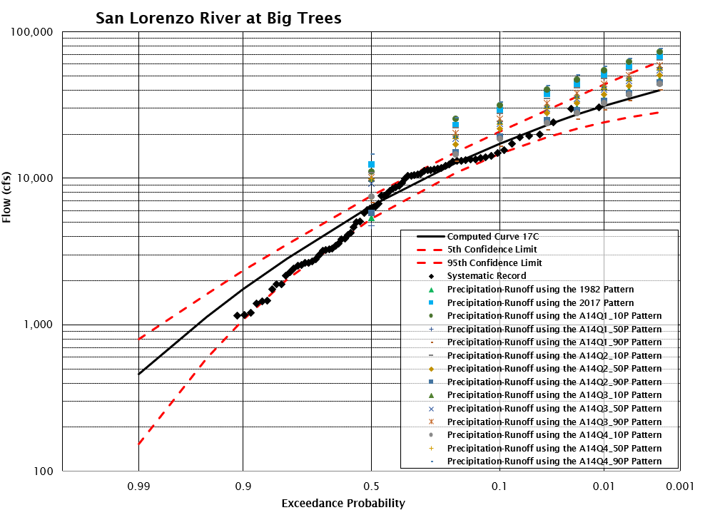
   AEP	Flow (cfs) for Pattern:
   	1982 Pattern	2017 Pattern	A14Q1_10P Pattern	A14Q1_50P Pattern	A14Q1_90P Pattern	A14Q2_10P Pattern	A14Q2_50P Pattern	A14Q2_90P Pattern	A14Q3_10P Pattern	A14Q3_50P Pattern	A14Q3_90P Pattern	A14Q4_10P Pattern	A14Q4_50P Pattern	A14Q4_90P Pattern
   0.5	5390	12394	11058	4723	6770	10840	7385	5780	9969	9211	10150	7539	9921	14558
   0.2	15048	22947	25405	15495	13001	22021	17055	15045	19370	18617	20288	14600	18514	25841
   0.1	19403	29027	31610	19700	16506	27576	21650	19234	24369	23463	25516	18538	23238	32763
   0.04	25273	37507	40261	25188	21240	35024	27744	24795	31026	29877	32444	23785	29689	42435
   0.02	29992	43937	47297	29434	25083	41068	32421	29070	36383	34927	37997	27882	35010	50172
   0.01	34999	50727	54636	33922	29192	47522	37389	33526	42116	40338	43921	32385	40706	57772
   0.005	39900	57703	62203	38727	33627	54389	42718	38297	48223	46111	50226	37185	46777	65583
   0.002	47028	67574	72661	45673	39995	63921	50290	45106	56887	54304	59175	44049	55413	76529

9. The following figure shows the HEC-HMS derived flow frequency results plotted along with the observed annual peak flow data and the Bulletin 17C flow frequency curve.

   

   As was noted earlier, the spread/uncertainty in the HEC-HMS flow frequency results is only due to the 24 hour storm temporal patterns, which are based on historical events. 

   

10. The flow frequency results computed by the HEC-HMS model were copied to an Excel spreadsheet and the flow values were converted to Log base 10. Then the variance and mean were computed for each AEP. The following table contains the variance and median flow (Log) from the HEC-HMS simulations. 

    AEP	Variance (Log Flow)	Median (Log Flow)
    0.5	0.0193	3.9804
    0.2	0.0081	4.2687
    0.1	0.0077	4.3683
    0.04	0.0076	4.4740
    0.02	0.0076	4.5437
    0.01	0.0074	4.6077
    0.005	0.0072	4.6669
    0.002	0.0069	4.7392

11. The weighted flow frequency curve was computed using equation 9-2 in Bulletin 17C. All flow and variance values were in log space when computing the weighted flow frequency curve. The following table and plot show the individual flow frequency curves and the weighted flow frequency curve. 

    AEP	Bulletin 17C Flow Frequency Curve (cfs)	Bulletin 17C Variance (Log Flow)	HEC-HMS Results Median Curve (cfs)	HEC-HMS Results Variance (Log Flow)	Weighted Flow Frequency Curve (cfs)
    0.99	463	0.0373	-	-	-
    0.95	1131	0.0151	-	-	-
    0.9	1746	0.0090	-	-	-
    0.8	2842	0.0050	-	-	-
    0.5	6451	0.0022	9559	0.0193	6711
    0.2	12734	0.0017	18565	0.0081	13601
    0.1	17248	0.0020	23350	0.0077	18363
    0.04	22973	0.0030	29783	0.0076	24721
    0.02	27118	0.0042	34968	0.0076	29683
    0.01	31096	0.0057	40521	0.0074	34900
    0.005	34902	0.0077	46443	0.0072	40422
    0.002	39664	0.0107	54856	0.0069	48282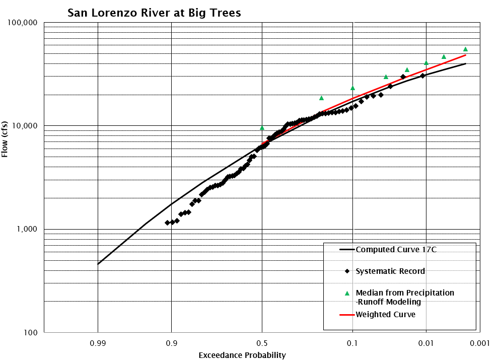

    
    
    

12. The weighted variance for each ordinate was computed using equation 9-3 in Bulletin 17C. Using the weighted variance, a 90% confidence interval (i.e. 5- and 95-percent confidence limits) was computed using equation 9-4 in Bulletin 17C. The following table and plot show the weighted variance, 5-, and 95-percent confidence limits.

    

    A t-value of 1.654 was used when computing the 90% confidence interval.

    AEP	Weighted Variance (log base 10)	5% Confidence Limit (cfs)	95% Confidence Limit (cfs)
    0.5	0.0019	7930	5679
    0.2	0.0014	15687	11792
    0.1	0.0016	21359	15788
    0.04	0.0021	29460	20745
    0.02	0.0027	36133	24385
    0.01	0.0032	43301	28129
    0.005	0.0037	50936	32078
    0.002	0.0042	61725	37767

    
    
    

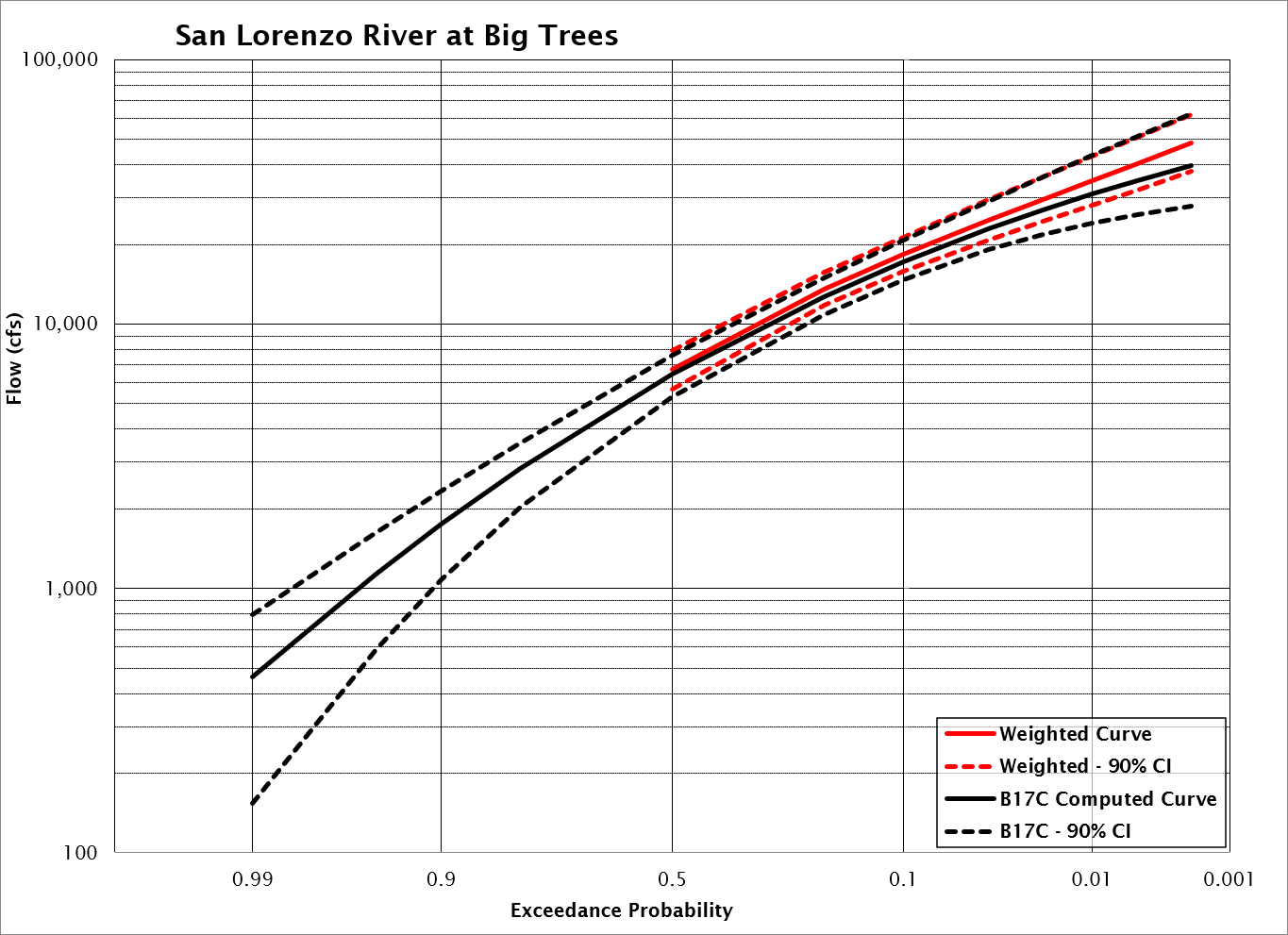
13. The B17C curve and weighted curve, along with their 90% confidence limits, were compared against one another.  The width of the 90% confidence limit was significantly reduced for rare AEP when precipitation-runoff results were combined with the B17C results, as shown in the following table and figure.

    AEP	B17C 90% Confidence Interval Width (cfs)	Weighted 90% Confidence Interval Width (cfs)
    0.5	2295	2252
    0.2	4113	3895
    0.1	6125	5571
    0.04	10114	8714
    0.02	14241	11748
    0.01	19311	15173
    0.005	25300	18858
    0.002	34596	23958