Download PDF
Download page Sampling NOAA Atlas 14 Temporal Patterns.
Sampling NOAA Atlas 14 Temporal Patterns
For applying temporal patterns in a deterministic way, return to Applying NOAA Atlas 14 Temporal Patterns.
Software Version
HEC-HMS version 4.12 was used to create this tutorial.
This tutorial should take approximately 30 minutes to complete.
Download the initial project files here:

Introduction
In hypothetical storm modeling, temporal patterns are far from certain. As part of each NOAA Atlas 14 volume, collections of statistically derived temporal patterns are provided and are categorized based on the quartile in which the greatest amount of precipitation fell and the cumulative probability of occurrence. This tutorial demonstrates how to randomly sample temporal patterns in an uncertainty analysis yielding probabilistic output that can serve as a form of sensitivity analysis with regard to potential temporal patterns.
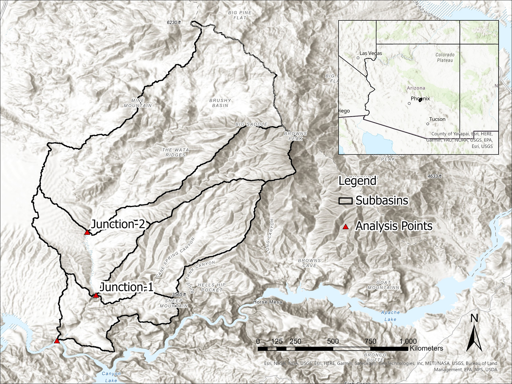
Study Area
Cottonwood Creek is a 64 square mile drainage the flows into the Salt River east of the Phoenix, AZ metropolitan area. This area falls within NOAA Atlas 14, Volume 1: Semiarid Southwest (Arizona, Southeast California, Nevada, New Mexico, Utah).
Create a Parameter Value Sample
In HEC-HMS parameter values can be sampled from a Parameter Value Sample Paired Data type. This process of creating a Parameter Value Sample for storm patterns and grid data has been expedited with the Parameter Value Sample Creator wizard.
Launch the Parameter Value Sample Creator wizard from Tools | Data | Atlas 14 | Parameter Value Sample Creator.
On step 1 of the wizard specify the Storm Pattern parameter.
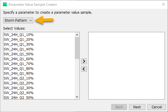
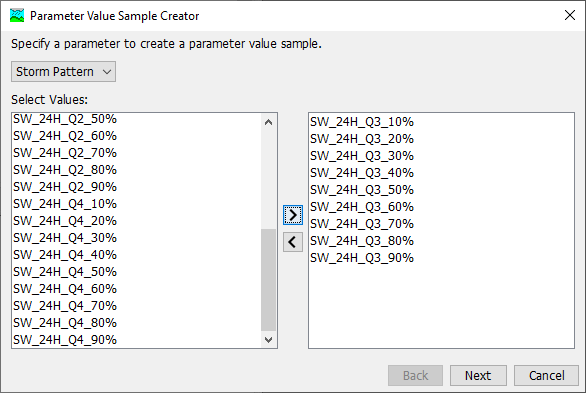
In this example we'll create a parameter value sample for Q3 curves. On step 1 of the wizard select just the Q3 curves.
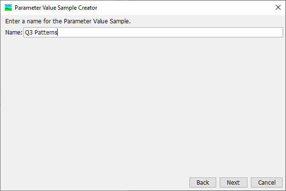
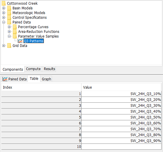
On step 2 of the wizard name the Parameter Value Sample "Q3 Patterns".
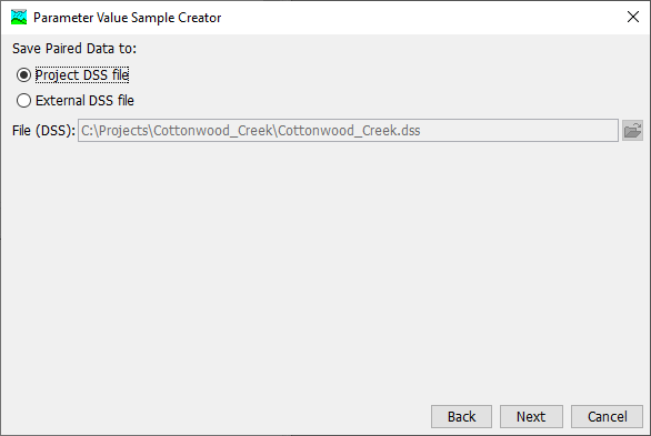
On step 3 of the wizard save the paired data to the project HEC-DSS file.
View the Parameter Value Sample from the Paired Data node in the Watershed Explorer.
Run Uncertainty Analysis
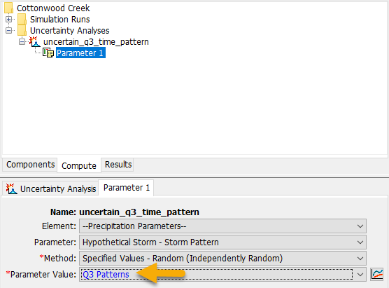
In the uncertain_time_parameter Uncertainty Analysis, select Parameter 1. In the Component Editor for Parameter 1, set the parameter value to Q3 Patterns.
Run the uncertain_time_parameter Uncertainty Analysis.
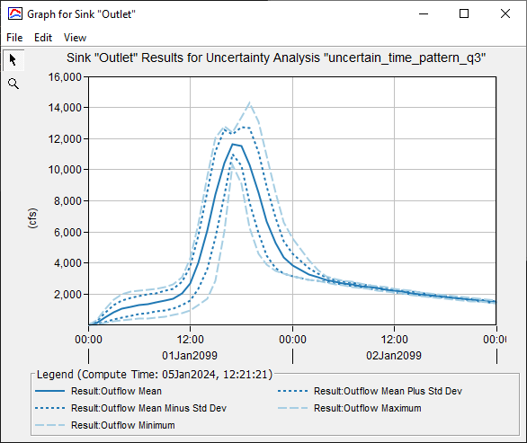
View probabilistic output for the Outlet.
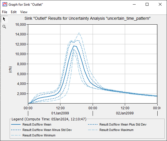
From the temporal pattern alone, peak flow magnitude at the outlet ranges from a minimum of approximately 10,000 cfs to a maximum of approximately 14,000 cfs. The average peak flow is between 11,000 and 12,000 cfs.
Run Additional Quartiles
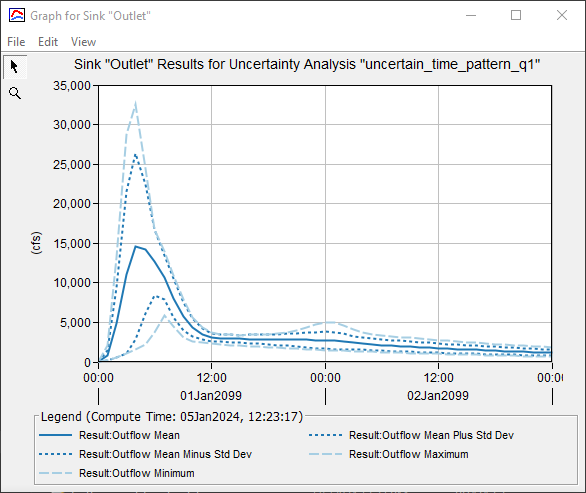
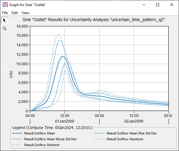
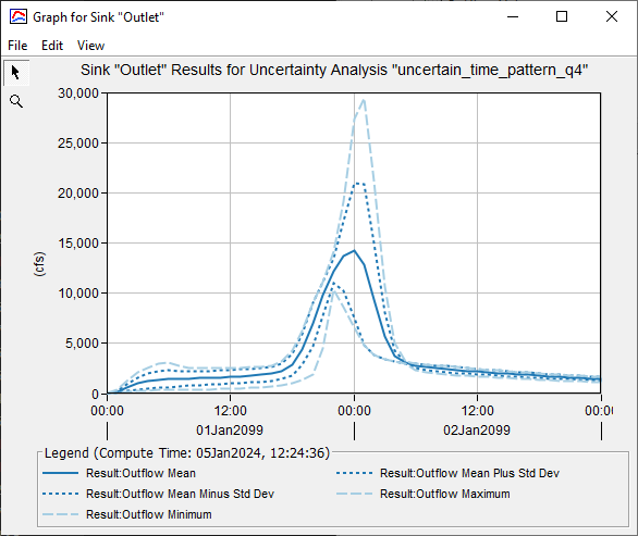
Additional Uncertainty Analyses were created for Quartile 1, 2, and 4 temporal patterns. From the results, the most intense precipitation pattern was observed in quartile 1, followed by quartile 2.
Quartile 1
Quartile 2
Quartile 3
Quartile 4
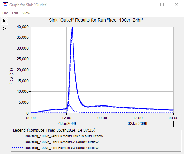
The frequency storm precipitation method in HEC-HMS uses the balanced hyetograph approach which nests frequency depth values for each duration and yields an unrealistic but maximally conservative (in terms of precipitation intensity) hyetograph. This same basin was tested using the frequency storm approach and yielded the following hydrograph at the outlet. For this basin, even the most extreme hypothetical precipitation event does not result in a hydrograph of the same magnitude of the balanced hyetograph approach (approximately 35,000 cfs vs approximately 40,000 cfs). The most extreme mean precipitation from the hypothetical storm approach is far less than that predicted using the balanced hyetograph (approximately 15,000 cfs vs approximately 40,000 cfs).
Summary
In this tutorial Parameter Value Samples for temporal patterns were created and sampled in an Uncertainty Analysis. This is a quick way to synthesize and apply all of the temporal pattern information that Atlas 14 provides.
Download the final project files here: