Download PDF
Download page Creating a Curve Number Grid and Computing Subbasin Average Curve Number Values.
Creating a Curve Number Grid and Computing Subbasin Average Curve Number Values
Last Modified: 2023-05-22 12:07:25.49
This tutorial demonstrates how to create a curve number grid and then compute the subbasin average curve number value.
Software Version
HEC-HMS version 4.11 beta 3 and ArcGIS Pro 2.9.3 were used to create this example. You can open the example HEC-HMS project with HEC-HMS 4.11 beta 3 or a newer version.Project Files
Example project can be found here:

Buffered Polygon of Total Watershed:
Introduction
This guide demonstrate how to create a curve number grid using land use and soil datasets and then computing the average curve number value for subbasins. The steps for creating the curve number grid are tailored for standard tools and options available in ArcGIS Pro 2.9.3. Once the curve number grid is computed in ArcGIS Pro, it is imported into an HEC-HMS project where HEC-HMS GIS tools are used to compute the subbasin average curve number. Soon, HEC-HMS will contain tools that can be used to create the curve number dataset from land use and soil datasets. For now, an external GIS is needed to create a curve number dataset.
Watershed
The Gallinas Creek watershed is located in Northern New Mexico. Gallinas Creek is a tributary of the Pecos River. An HEC-HMS model of the upper portion of the Gallinas Creek watershed was created in response to the Calf Canyon / Hermits Peak fires that burned over 300,000 acres in the Sangre de Cristo Mountains, including a significant portion of the Gallinas Creek watershed upstream of Las Vegas, NM.
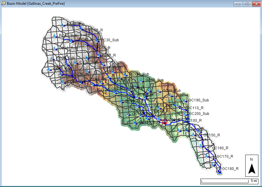
The follow figure shows the subbasin delineation defined for the watershed. Small subbasins, less than 3 square miles, were delineated in an effort to estimate debris and sediment from burned areas in the watershed. The red element in the figure is the Gallinas Creek near Montezuma USGS gage location, 08380500.
Datasets for Creating the Curve Number Grid
The 2019 National Land Cover Database (NLCD) dataset was used for the example. You can download the GIS files from - https://www.mrlc.gov/data/nlcd-2019-land-cover-conus. The NLCD dataset covers the continental United States at a 30 meter resolution, and the dataset has been projected into an equal area projection. Each raster cell value represents a land cover type. The attached PDF provides a description for each of the land cover types -
.
The Gridded Soil Survey Geographic (gSSURGO) database was used for this example. The database contains a GIS layer of soil polygons and many attribute tables describing the properties for each soil polygon. You can download the database files for each state from - https://nrcs.app.box.com/v/soils/folder/148414960239. The Hydrologic Soil Group was used to compute the curve number, the hydrologic soil group is contained in the Component table within the gSSURGO database. The attached PDF provides a description for each hydrologic soil group -
.
Datasets
The datasets used for this example were used to illustrate a process. There are many other land use and soil datasets available. You should choose the appropriate datasets for your analysis.
Land Use and Soil Lookup Table
A curve number is estimated using a lookup table that assigns a curve number to each combination of land use type and hydrologic soil group. The table below was used for this example, values in green are the curve numbers. There are many resources available for defining curve numbers given land use, soil types, and antecedent moisture conditions. Use the appropriate curve number lookup table for your application.
NLCD 2019 | Hydrologic Soil Group | ||||
|---|---|---|---|---|---|
Land Use Description | Land Use Value | A | B | C | D |
Open Water | 11 | 98 | 98 | 98 | 98 |
Developed, Open Space | 21 | 49 | 69 | 79 | 84 |
Developed, Low Intensity | 22 | 57 | 72 | 81 | 86 |
Developed, Medium Intensity | 23 | 61 | 75 | 83 | 87 |
Developed High Intensity | 24 | 81 | 88 | 91 | 93 |
Barren Land (Rock/Sand/Clay) | 31 | 78 | 86 | 91 | 93 |
Deciduous Forest | 41 | 45 | 66 | 77 | 83 |
Evergreen Forest | 42 | 25 | 55 | 70 | 77 |
Mixed Forest | 43 | 36 | 60 | 73 | 79 |
Shrub/Scrub | 52 | 55 | 72 | 81 | 86 |
Grassland/Herbaceous | 71 | 50 | 69 | 79 | 84 |
Pasture/Hay | 81 | 49 | 69 | 79 | 84 |
Cultivated Crops | 82 | 67 | 78 | 85 | 89 |
Woody Wetlands | 90 | 30 | 58 | 71 | 78 |
Emergent Herbaceous Wetlands | 95 | 30 | 58 | 71 | 78 |
Steps for Processing the NLCD 2019 Dataset
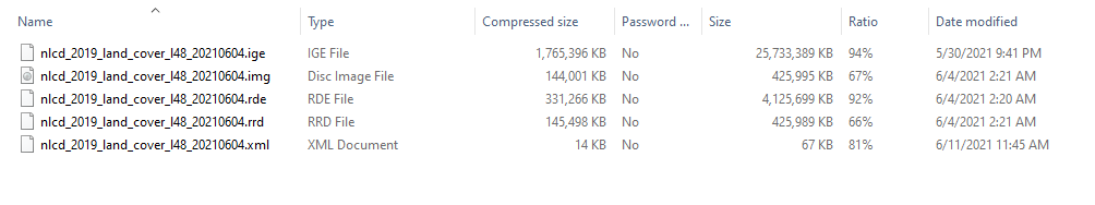
The figure below shows the files contained in the NLCD 2019 dataset. Since this is a national coverage, we will need to clip the data to the buffered watershed extents to reduce file sizes and processing times. I also like to project all data into a common projection. In this example, the GIS datasets are projected into the NAD_1983_2011_StatePlane_New_Mexico_East_FIPS_3001_Ft_US projection since this is the projection defined within the HEC-HMS project.
- Add the nlcd_2019_land_cover_l48_20210604.img file to an ArcMap Pro project.
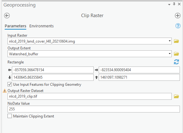
- Open the Geoprocessing Tool and search for the Clip Raster tool. As shown in the figure below:
- Choose the nlcd_2019_land_cover_l48_20210604.img file as the Input Raster.
- Choose the Watershed_buffer layer to set the Output Extent (this polygon layer was created by buffering the HEC-HMS subbasin elements by 1000 feet).
- Check the box to Use Input Features for Clipping Geometry.
- Enter a name for the Output Raster Dataset, nlcd_2019_clip.tif. Enter a file extension of "tif" so that the new raster will be in GeoTIFF format.
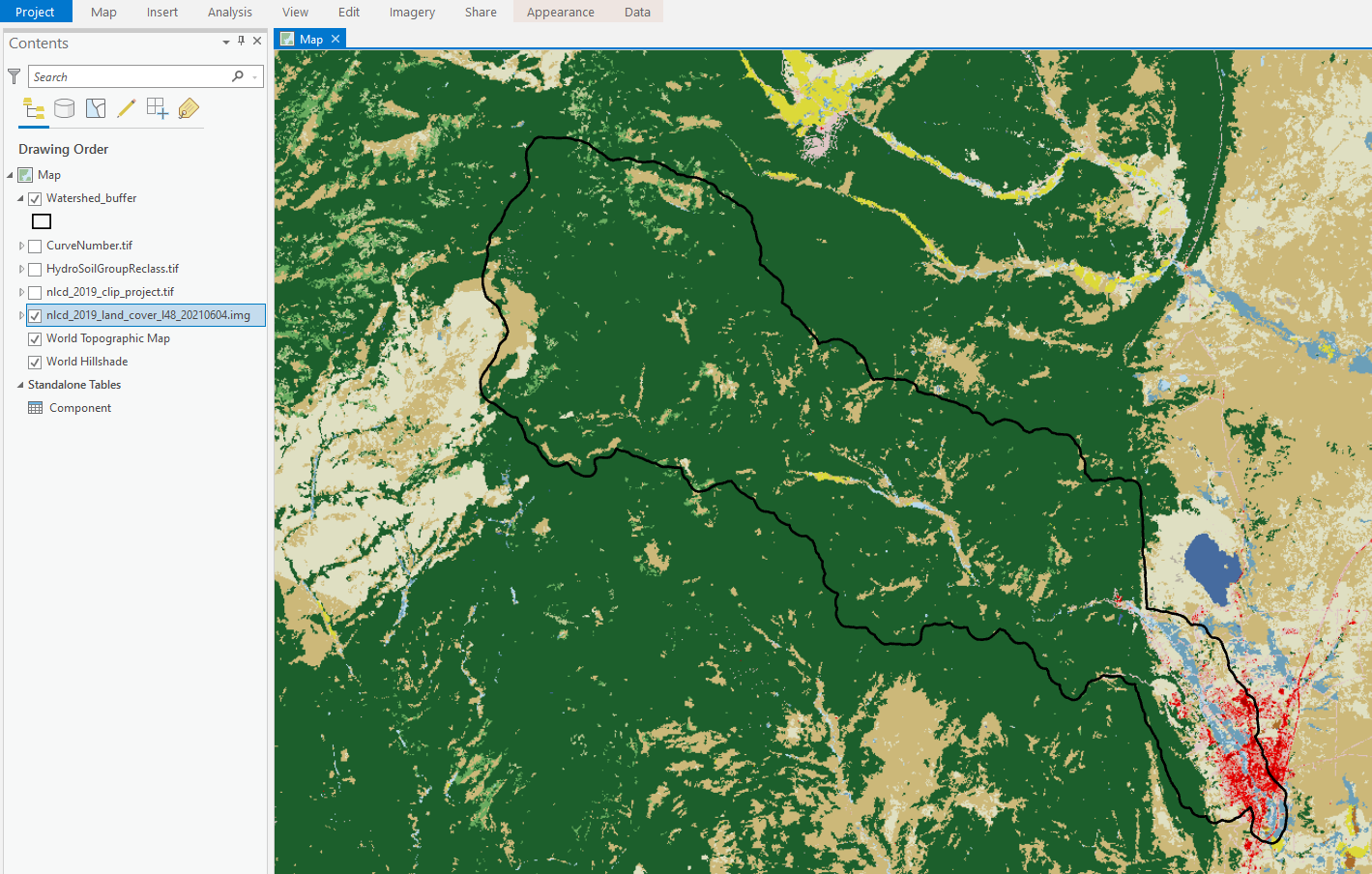
- The new NLCD 2019 raster should be added to your ArcMap Pro project, you should notice the land use data is only defined for the watershed area.
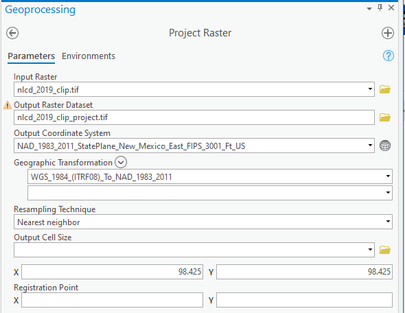
- Open the Geoprocessing Tool and search for the Project Raster tool. As shown in the figure below:
- Choose the nlcd_2019_clip.tif file as the Input Raster.
- Enter a name for the Output Raster Dataset, nlcd_2019_clip_project.tif. Enter a file extension of "tif" so that the new raster will be in GeoTIFF format.
- Choose the new coordinate system. In this example, New Mexico State Plane East was used. The horizontal units for this projection are feet.
- Make sure the Nearest neighbor Resampling Technique is selected.
- You can change the output cell size if needed. In this example the cell size was not changed, 30 meters = 98.425 feet.
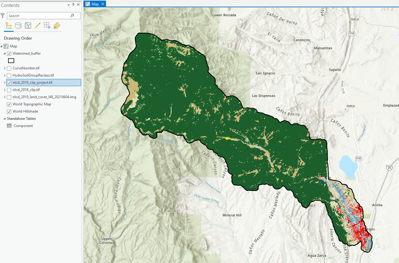
- The following figure shows the final NLCD 2019 dataset for the example watershed. A majority of the Land Use is classified as 42, which is Evergreen Forest.
Steps for Processing the New Mexico gSSURGO Dataset
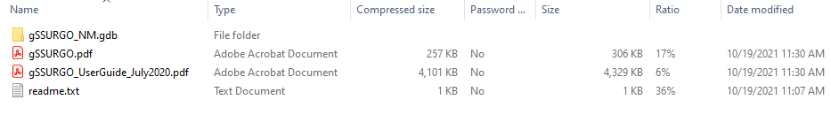
The figure below shows the files contained in the New Mexico gSSURGO dataset. The Geodatabase file contains vector polygons defining consistent soil types and many attribute tables with information about each soil type. We will follow the same steps to clip and project the soil dataset. Some additional work is needed to assign a hydrologic soil group to each soil polygon layer. I like to work with raster datasets rather than vector datasets, so we will convert the soil polygon dataset to a raster.
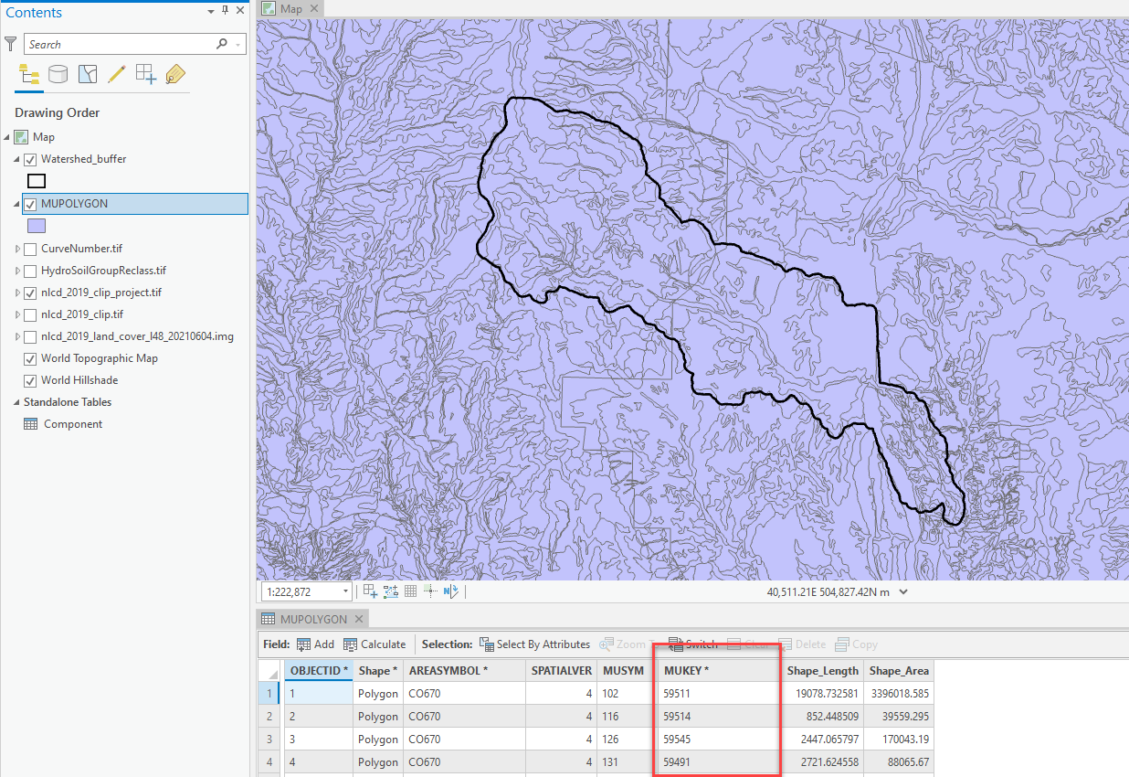
- Add the MUPOLYGON dataset to an ArcMap Pro project, the MUPOLYGON layer is located within the gSSURGO geodatabase. The figure below shows the attribute table for the MUPOLYGON layer. Notice the MUKEY attribute. The MUKEY will be used to join information from other tables in the gSSURGO geodatabase.
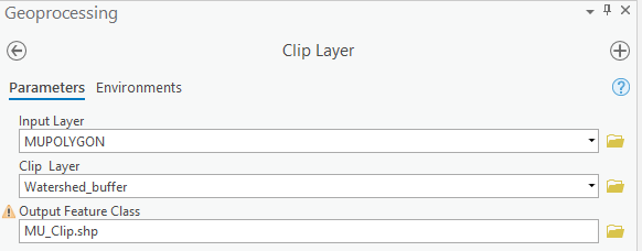
- Open the Geoprocessing Tool and search for the Clip Layer tool. As shown in the figure below:
- Choose the MUPOLYGON layer as the Input Layer.
- Choose the Watershed_buffer layer as the Clip Layer.
- Enter a name for the Output Raster Class, MU_Clip.shp. Enter a file extension of "shp" so that the new layer will be in shapefile format.
- The new soil layer should be added to your ArcMap Pro project, you should notice the soil polygons are only defined for the watershed area.
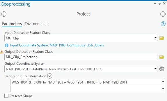
- Open the Geoprocessing Tool and search for the Project tool. As shown in the figure below:
- Choose the MU_Clip file as the Input Feature Class.
- Enter a name for the Output Feature Class, MU_Clip_Project.shp.
- Choose the new coordinate system. In this example New Mexico State Plane East was used.
- A Geographic Transformation was automatically selected.
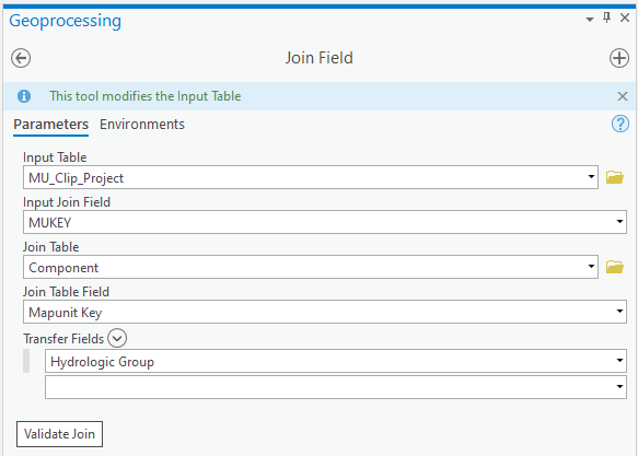
- Open the Geoprocessing Tool and search for the Join Field tool. As shown in the figure below:
- The Input Table is the attribute table from the MU_Clip_Project shapefile.
- The attribute in the MU_Clip_Project table with the common data for the join is the MUKEY field.
- The table with information we want to add to the MU_Clip_Project attribute table is the Component table. The Component table is one of the tables in the gSSURGO_NM.gdb file.
- The Component table has an attribute labeled Mapunit Key, which is similar to the MUKEY field in the MU_Clip_Project shapefile.
- Choose the Hydrologic Group attribute field to transfer from the Component table to the MU_Clip_Project attribute table.
- After running the Join Field tool, you should see a new attribute in the MU_Clip_Project shapefile as shown in the figure below. The "hydgrp" field was added to the attribute table.
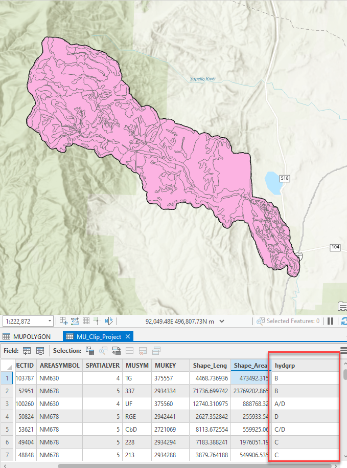
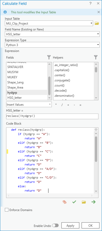
- We need to remove any hydrologic soil groups that are not the standard A, B, C, or D groups. You will notice some combinations of soil groups, like A/D. The dual case soil groups are made up of land that is drained and undrained. You will also notice some of the soils will have a soil group of "0" defined as well. A conservative approach is to assign a hydrologic soil group of D to all dual soil groups and those soils with no soil group defined. The following steps show how to add a new attribute and process the hydrologic soil groups so that there is only one standard hydrologic soil group per soil polygon.
- Add a new attribute to the table as shown below.
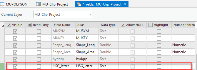
- Use the Calculate Field tool to transfer information from the hydgrp field and convert duel or non standard values. As shown below, a Code Block was used to define the logic for modifying the duel hydrologic soil groups. There were no "B/D" soil groups within the watershed boundary.
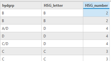
The following figure shows a portion of the updated attribute table.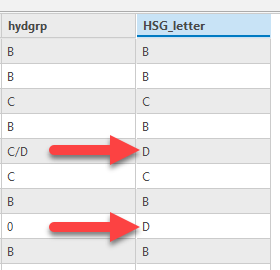
- For later processing steps, we need to represent the hydrologic soil groups using numeric values instead of letters A, B, C, and D. Follow the steps shown above and add another attribute to the MU_Clip_Project shapefile, HSG_number, and assign hydrologic soil group A a value of 1, hydrologic soil group B a value of 2, hydrologic soil group C a value of 3, and hydrologic soil group D a value of 4. The following figure shows how the Calculate Field tool was used to convert hydrologic soil groups to numeric values.
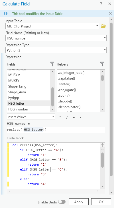
- Add a new attribute to the table as shown below.
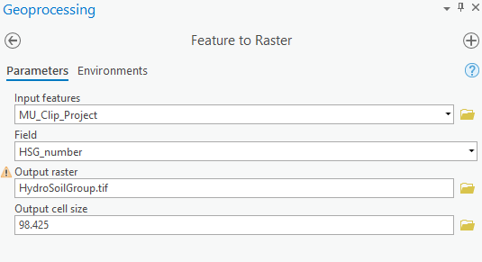
- The last step is to convert the polygon soil layer to a raster dataset. Open the Geoprocessing Tool and search for the Feature to Raster tool. As shown in the figure below:
- The Input features is the MU_Clip_Project shapefile.
- The attribute Field is the HSG_number field.
- The Output raster was named HydroSoilGroup.tif. Enter a file extension of "tif" so that the new raster will be in GeoTIFF format.
- An Output cell size of 98.425 feet was specified to match the NLCD 2019 cell size.
Create the Curve Number Raster
Now that we have land use and soil raster datesets, we can use the Raster Calculator to compute a curve number dataset. The Raster Calculator will create a new raster dataset by evaluating existing raster datasets.
- Open the Geoprocessing Tool and search for the Raster Calculator tool. As shown in the figure below, there is an area to define a logic expression and you must enter the name of the Output raster. The Output raster was named CurveNumber.tif. Enter a file extension of "tif" so that the new raster will be in GeoTIFF format.
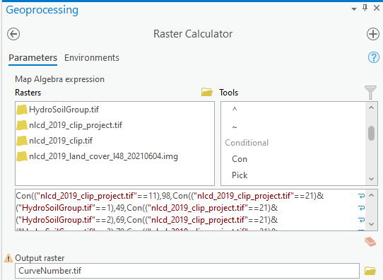
- The Raster Calculator has a conditional statement option that is similar to an If statement. For example, the statement Con(("nlcd_2019_clip_project.tif"==11),98,0) is similar to stating: If a grid cell in the nlcd_2019_clip_project.tif raster = 11, then assign a value of 98 to the new raster, else, assign a value of 0 to the new raster. The portion of the logic expression in the red box shown below shows that two raster datasets can be evaluated within the conditional statement. In this example, grid cells that have a NLCD 2019 value of 21 (Developed, Open Space) and Hydrologic Soil Group of 3 (C) will be assigned a value of 79.
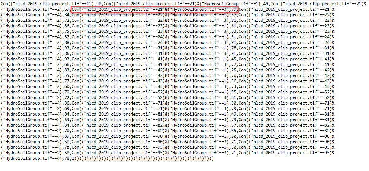
- You can download a text file that has the formula used in this example:
- You can copy and paste the formula if following along. You will need to modify the formula if you have a different lookup table or if you named your land use or soil datasets differently.
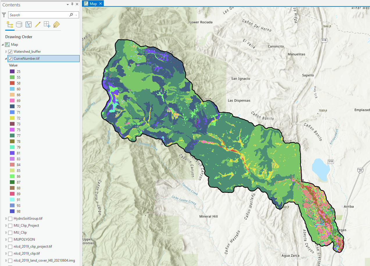
- The following figure shows the Curve Number raster created by the Raster Calculator.
Use HEC-HMS to Compute the Subbasin Average Curve Number
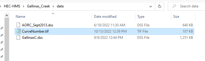
- Copy the CurveNumber.tif file created in the previous step and place it in the Gallinas Creek HEC-HMS project directory, within the data folder.
- Open the Gallinas Creek HEC-HMS project.
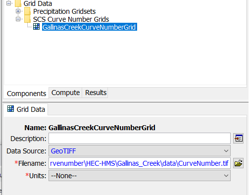
- Open the Grid Data Manager and add a new SCS Curve Number Grid named GallinasCreekCurveNumberGrid to the project.
- Navigate to the Grid Data folder, expand the Watershed Explorer and select the GallinasCreekCurveNumberGrid node to open the Component Editor. Choose a Data Source of GeoTiff, and then select the file using the filename chooser button. The component editor should be similar to the figure below.
- Select the Gallinas_Creek_PreFire basin model to open the basin model in the desktop area.
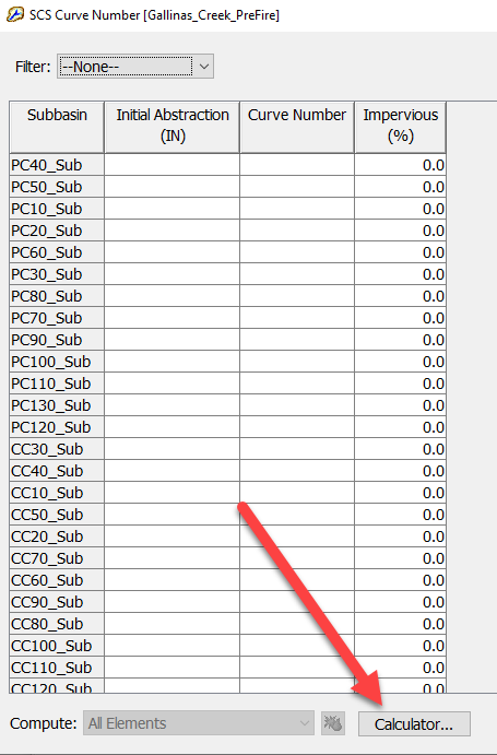
- Select the Parameters | Loss | SCS Curve Number to open the SCS Curve Number Global Editor.
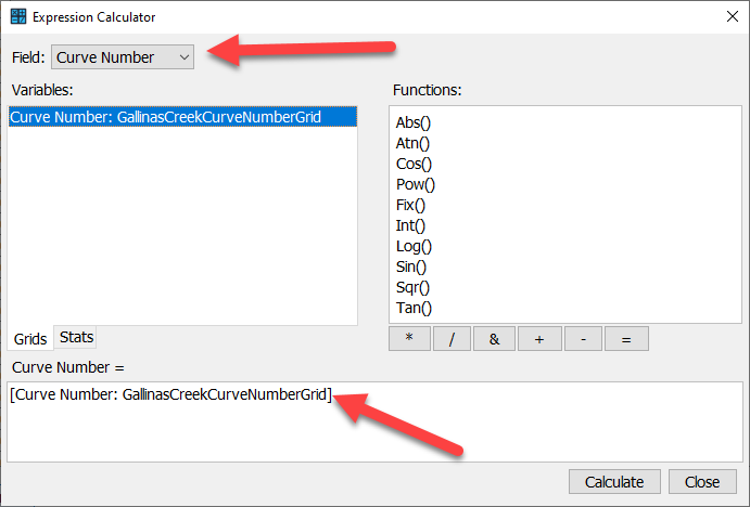
- Click the Calculator button at the bottom of the SCS Curve Number Global Editor.
- Within the Expression Calculator, choose the Curve Number field, and then double click the GallinasCreekCUrveNumberGrid in the Variables list to add it to the expression at the bottom of the calculator. Click the Calculate button.
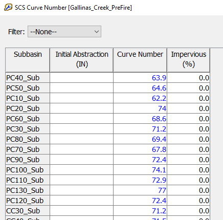
- As shown below, you will notice that the program automatically computes the average curve number value for each subbasin.
Take a look at the following tutorial if you are interested in the Gridded SCS Curve Number option - Importing Gridded SCS Curve Number in HEC-HMS.
Final Project Files