Download PDF
Download page Preparing Terrain Data for HEC-HMS using QGIS.
Preparing Terrain Data for HEC-HMS using QGIS
Overview
In this tutorial we use free open-source GIS software QGIS to prepare terrain data in the form of Digital Elevation Model (DEM) raster from open-source elevation and watershed boundary data (see the tutorial on Downloading Elevation and Watershed Boundary Data). Other GIS applications (e.g. ArcMap) can be used instead of QGIS. Refer to Downloading and Preparing Terrain Data for HEC-HMS Using ArcMap for directions. A DEM is a representation of the bare ground topography (elevations) excluding trees, buildings, and any other surface objects. We will use it as an input to HEC-HMS to create a terrain dataset, which can then be loaded into a Basin Model for hydrologic analysis (see Creating and Linking Terrain Data into a Basin Model tutorial). We will use the watershed boundary to clip the extent of the terrain raster for smaller file sizes and faster processing.
Background
The watershed used in this example is the 140 square mile East Branch Brandywine Creek watershed in Pennsylvania.

Process terrain data in QGIS
In this example we merge, clip and project the DEM file in QGIS Version 3.16.3.
Step 1: Add terrain raster data
- Open QGIS and start a new project Project | New (1) or open an existing project Project | Open (2).

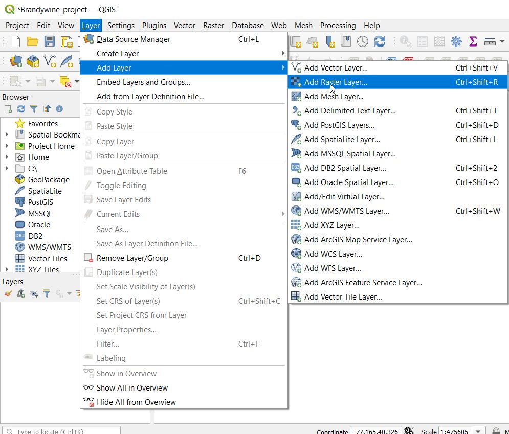
- Select Layer | Add Layer | Add Raster Layer to add a raster layer with terrain data created in the previous step.
- Select the File Source type (1).
- Browse to the terrain raster's location (2) and click Add (3). Repeat for the second terrain raster.

You can also add a basemap for reference by browsing to the XYZ Tiles and double-clicking on one of the available options.

Step 2: Merge multiple terrain files
This step is only necessary if you downloaded more than one terrain data set (two in this example).
- Navigate to Raster | Miscellaneous | Merge.
- Select input terrain rasters (1).
- Set Output data type to Float32 (2).
- Under Advanced Parameters, assign the input "nodata" value to match the value specified in the input dataset's metadata (-999999 for the USGS terrain) (3) and specify the output "nodata" value (e.g. -9999) (4)
- Select Save to file from the drop down menu in the Merged browse box (5), browse to the output file location and save the merged file with *.tif extension
- Check Open output file after running algorithm option (6) and click Run

- The merged raster is now added to the Layers tree
Step 3: Import watershed boundary data
Add watershed boundary data from previous steps (HUC-10 level shapefile is used in this example) to your project.
- Select Layer | Add Layer | Add Vector Layer
- Select the File Source type (1), open the watershed boundary folder and browse to select the WBDHU10.shp file and click Add

- The watershed boundary is now added to the Layers tree
Step 4: Reproject terrain rasters
Terrain data must by in a projected coordinate reference system (CRS) for hydrologic modeling. For example, the USA Albers Equal Area Conic USGS Version Linear Unit: Foot_US (0.3048006096012192) is routinely used by USACE within hydrologic modeling applications because this CRS preserves area, which is crucial for hydrologic modeling.
Do NOT use an unprojected CRS, such as Geographic.
- Browse to Raster | Projections | Warp (Reproject) dialog
- Select Input layer (the merged terrain raster) (1)
- Set Source CRS to match the input layer's CRS (2), which can be found in the metadata section for the imported terrain
- Be sure to use either the Bilinear or Cubic resampling method (3)
- Set no data values to -9999 (4)
- Click on Save to File dropdown menu and browse to file location to save the reprojected raster in *.tif format (4)
Click on the browsing icon for Target CRS (5) to open the Coordinate Reference System Selector dialog for the output raster

Un-select the checkbox for No CRS (or unknown / non-Earth projection) (1)
Browse to Projected Coordinate Systems | Albers Equal Area to select Canada_Albers_Equal_Area_Conic (ESRI: 102001) (2) or an appropriate local projection and click Ok.

Step 5: Reproject watershed boundary shapefile
Project the watershed boundary shapefile to the same CRS as the terrain data.
- Browse to Vector | Data Management Tools | Reproject Layer to open the Reproject Layer dialog
- Select the watershed boundary shapefile as the input layer (1)
- Click on Save to File dropdown menu (2) to save reprojected layer in *.shp format
- Click on the earth icon (3) next to the Target CRS field to select the output projection

- Browse to Projected Coordinate Systems | Albers Equal Area to select Canada_Albers_Equal_Area_Conic (ESRI: 102001) (1) and click Ok
- The coordinate system should also be available under Recently Used Coordinate Reference Systems (2)

Step 6: Set project CRS to match reprojected layers
- From Project | Properties | CRS (1) browse to Projected Coordinate Systems | Albers Equal Area to select Canada_Albers_Equal_Area_Conic (ESRI: 102001) (2) and click Ok.
- Choose the default reprojection method if prompted

Step 7: Extract the watershed boundary shapefile
We will buffer this shapefile and use it as a boundary to clip the terrain raster in the following steps.
- Using the Identify Features (1) and Select Features (2) tools, select the watershed of interest (East Branch Brandywine Creek in this example) from the reprojected WBDHU10 watershed boundary shapefile layer created in previous step
- Right click on the shapefile layer in the tree (3) and select Export | Save Selected Feature as from the dropdown menu.

- Enter the name and location for the extracted shapefile (1)
- Save with the same equal area projection as the reprojected terrain raster (2)
- Check Save only selected features (3) and Add Saved File to Map (4) boxes

Step 8: Buffer the watershed boundary shapefile
Buffer the area of interest by two miles (3 kilometers) to avoid edge effects within the area of interest and save the buffered shapefile.
- Navigate to Vector | Geoprocessing Tools | Buffer to open the Buffer dialog
- Set input layer to the watershed boundary (1)
- Set distance to 2 miles (2)
- Select Save to File from the dropdown menu (3) and save the buffered boundary in *.shp format

The buffered watershed boundary layer is added to the map.

Step 9: Clip projected terrain raster with the buffered watershed boundary
Clip the reprojected terrain raster created in Step 4 using the buffered boundary shapefile from the previous step. This step helps reduce the size of the terrain model and subsequent processing time.
- Open Clip Raster by Mask Layer dialog from Raster | Extraction menu
- Select the merged reprojected terrain raster as the input layer (1) and the buffered watershed boundary as the mask layer (2)
- Set the Source CRS and Target CRS to the equal area projection matching the reprojected terrain raster (3)
- Set the "nodata" value to -9999 (4) (if left empty, the values outside of the cutting boundary will be set to zero and displayed by default)
- Check boxes to Match the extent of the clipped raster to the extent of the mask layer (5) and Keep resolution of input raster (6)
- Save the clipped raster in *.tif format (7).

The clipped terrain layer is now added to the map, as shown below.

Step 10: Check for no data values
HEC-HMS delineation tools require a continuous surface with no interior raster cells containing missing elevation values. We can check for and replace missing elevation data with mean values using the Raster Calculator
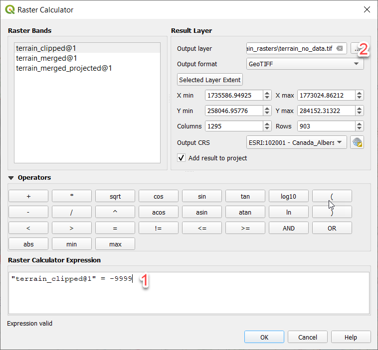
- Navigate to Raster | Raster Calculator
- Double click on the clipped raster layer to add the raster name to the Raster Calculator Expression (1), then enter = -9999. This expression will result in a raster with "nodata" cells set to one and the remaining cells set to zero.
- Save the "nodata" raster as a separate *.tif file (2)
- Check the new raster layer to see if any interior grid cells have a value of 1. If they do have a value of 1, then that grid cell is missing an elevation value and needs to be filled in with an appropriate elevation value. The terrain raster in this example has no missing data.
Step 11: Replace "nodata" values
This step is only required if internal grid cells with missing data were identified in previous step. You can fill out the missing values by extrapolating from the surrounding raster cells using the open source geospatial data abstraction library (GDAL) tools from within QGIS. The algorithm uses inverse distance weighting over the user-defined number of cells.
- Go to Processing | Toolbox | GDAL | Raster analysis | Fill nodata
- Select the clipped terrain as the input layer
- Keep default parameters for the number of pixels (cells) to use in the interpolation (10) and number of smoothing iterations (0)
- Save the filled raster in *.tif format.
Import the new terrain dataset within an HEC-HMS project
Step 1: Import the final terrain raster as new Terrain Data in HEC-HMS.
- Open or create a new project in HEC-HMS.
- Set the Default Unit System (U.S. Customary in this example)

- From the Components menu, select Terrain Data Manager and create a new terrain dataset

- Click Next and browse to the final terrain *.tif file that was created in the previous steps (1).
Set the vertical units to match the vertical units in the terrain raster (meters in this example) (2).

Step 2: Link the terrain dataset to a basin model.
- In HEC-HMS, go to Components => Basin Model Manager to create a new basin model.

- Click on the new basin model (Brandywine_basin) in the Watershed Explorer (1)
- Within the Component Editor (lower left corner), select the terrain dataset (Brandywine_DEM) within the Terrain Data drop down menu (2)
- Click Save (3)

- If the Basin Model does not have a defined coordinate system, a popup menu will be shown
- Choose Skip to adopt CRS from the referenced GIS data (the terrain *.tif file). This option should be used 99% of the time. Use the other option to choose a CRS from an existing file.

The terrain data will now appear in the map model map and can be used to delineate elements, compute grid cells, and compute subbasin and reach characteristics.
