Download PDF
Download page Using the Parameter Expression Calculator to Estimate Model Parameters.
Using the Parameter Expression Calculator to Estimate Model Parameters
This tutorial was completed using HEC-HMS 4.10 beta 6.
Download the initial project files here - Initial_ExampleProject.zip
Introduction
The purpose of this tutorial is to show how the new parameter expression calculator can be used to estimate model parameters using either physical characteristics of subbasins or readily available GIS datasets. The new parameter expression calculator option is available from a few of the global parameter editors, including the Clark and S-Graph transform editors and the Deficit and Constant and Green and Ampt loss editors. The parameter expression calculator will be added to other global editors for future software releases. The parameter expression calculator will compute subbasin average parameter values from raster datasets (parameter grids). The program uses the zonal statics GIS function to compute subbasin average parameter values when raster datasets are used.
Watershed Description and Background
The area modeled in this tutorial is part of the Coyote Creek watershed in Northern California. See the following tutorial for information about the watershed - Comparing HEC-HMS Discretization and Transform Options. In summary, an HEC-HMS model was developed for part of the Coyote Creek watershed, the upper 109 square miles. Observed precipitation and flow data were available to calibrate the model. For this tutorial, the subbasin elements were configured to use the Green and Ampt loss method, the Clark transform method, and the Linear Reservoir baseflow method. As described below, the parameter expression calculator was used to estimate some of the Clark transform and Green and Ampt loss parameters.
Soil and landuse GIS datasets were used to estimate the Green and Ampt parameters. After the GIS datasets were gathered, they were re-projected into a consistent projection (the same projection set in the HEC-HMS basin model). The parameter expression calculator in HEC-HMS works with raster datasets (HEC-HMS parameter grids). Therefore, vector landuse and soil GIS data must be converted to raster datasets. A separate raster dataset was created for each parameter, moisture deficit, saturated hydraulic conductivity, wetting front suction, and percent impervious area. There are many GIS datasets available and methods for processing them. The following is one method to created the needed parameter grids in a format that can be used within HEC-HMS.
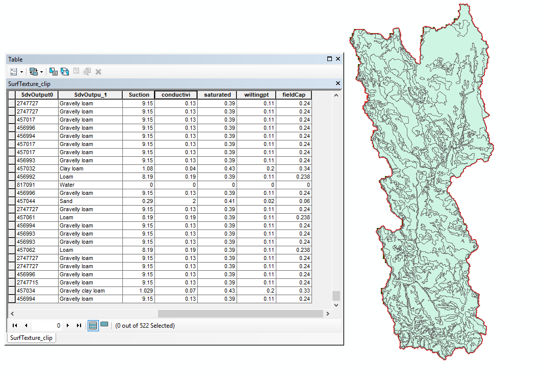
The figure below shows a vector (polygon) soil layer for the Coyote Creek watershed. The surface soil texture was identified for each polygon. Then, properties were entered for each surface soil texture type, wetting front suction, saturated hydraulic conductivity, saturated content, wilting point, and field capacity. This information was added to the soil layer's attribute table using editing tools and the table join tool (each polygon contains a key/code that can be used to join information that is specific to each soil polygon).
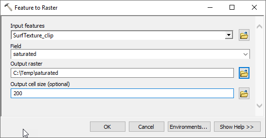
The following figure shows the Feature to Raster tool in ArcGIS. This tool will create a new raster dataset using values in the select field (attribute). In the example shown, the saturated content attribute was selected and a raster with a cell size of 200 meters will be created. The output cell size does not have to match the cell size used when discretizing HEC-HMS subbasins.
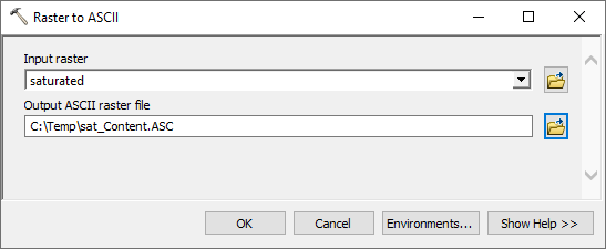
HEC-HMS accepts both ASCII and GeoTIFF file formats for parameter grids. The ArcGIS Raster to ASCII tool, see below, can be used to convert a raster from ESRI Grid format to ASCII format. Once the ASCII file is created, copy it (along with the projection file) to the HEC-HMS project directory. HEC-HMS will use relative pathnames for external files when they are located within the project directory (which makes it easy to transfer the project from one computer to another).
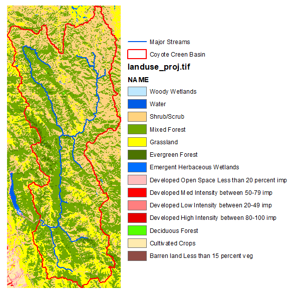
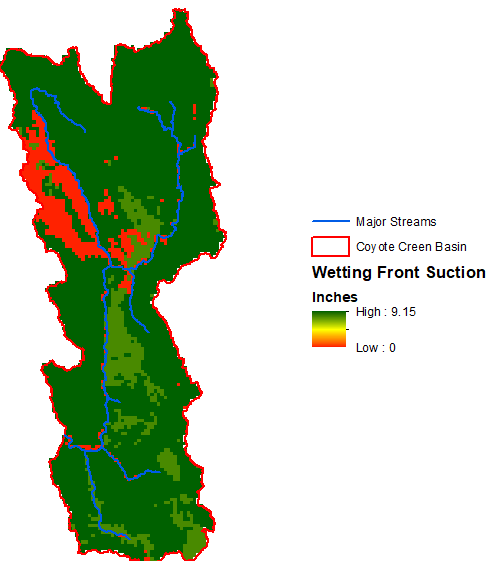
The following figures show the landuse and wetting front suction GIS datasets for the Coyote Creek watershed. The percent impervious area was estimated for each landuse type using the Reclassify tool in ArcGIS. Since the watershed is mostly shrub and mixed forest land, the percent impervious area is very small throughout the watershed. The SSURGO dataset was used to create raster layers for the saturated hydraulic conductivity and wetting front suction. The moisture deficit was estimate as a fraction of the soil's porosity. The moisture deficit reflects the soil moisture at the beginning of a model simulation.
 ++
++
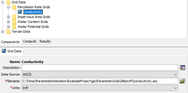
As shown below, HEC-HMS 4.10 has an option to choose an ASCII or GeoTIFF Data Source for parameter grids, in addition to the HEC-DSS format. In order to use the parameter grids in the parameter expression calculator, the parameter grids must be added to the project in either the ASCII or GeoTIFF formats. For this tutorial, a percolation rate, impervious area, water content, and water potential grids have already been added to the project in the ASCII format. The ASCII files are located in the ...\ExampleProject\gis\ParameterGrids\Albersft directory. A copy of the ESRI grids used to create these ASCII files are located in the ...\ExampleProject\gis\ArcDatasets directory.
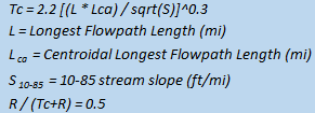
The Clark time of concentration and storage coefficient parameters can be estimated using the following equations (the coefficient and exponent should be determined/calibrated regionally). The equation for the time of concentration relates the longest flow path, centroidal flow path, and 10-85 flow path slope to the time of concentration. HEC-HMS 4.10 will compute these physical characteristics for subbasin elements. In order for the program to compute subbasin characteristics, the subbasin elements must be delineated using the GIS delineation tools in HEC-HMS. Subbasin characteristics can still be computed for those existing projects that were completed before the GIS delineation tools in HEC-HMS were made available. The subbasin elements must be georeferenced using a shapefile and then terrain data must be added to the basin model and the GIS→Preprocess Drainage and GIS→Identify Streams steps completed.
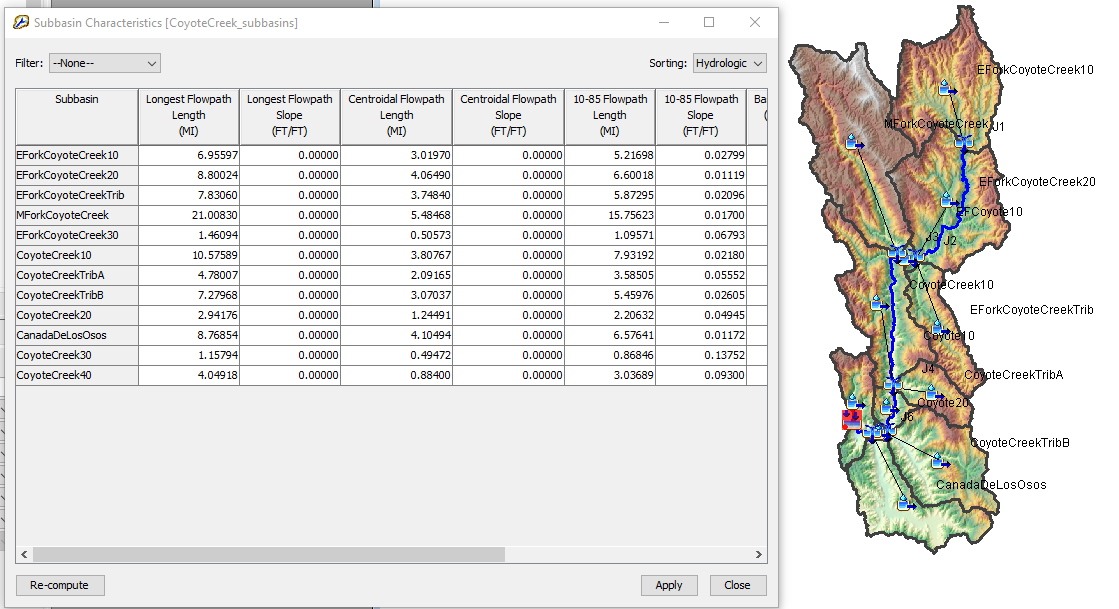
The following figure shows the subbasin characteristics for the Coyote Creek watershed. You can see this information from the Parameters→Characteristics→Subbasin menu option.
Using the Parameter Estimation Calculator to Estimate the Time of Concentration
- Open the example project attached to this tutorial. Open the CoyoteCreek_subbasins basin model.
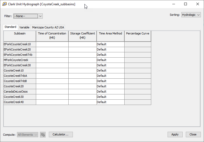
- Select the Parameters→Transform→Clark Unit Hydrograph menu option to open the Clark Unit Hydrograph global editor as shown below.
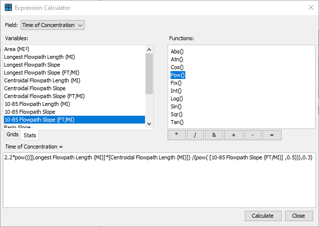
- Click the Calculator... button at the bottom of the global editor. The following figure shows the Expression Calculator. Select the Time of Concentration in the upper left. Then make sure the Stats tab is selected in the Variables panel. The stats tab is linked to the subbasin characteristics. The equation panel shows the equation entered to estimate the time of concentration. After recreating this equation, click the Calculate button and the the program will add the computed values to the global editor.
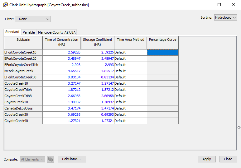
- Assuming an R/(R+TC) relationship of 0.5 means R is equal to TC. Within the global editor, copy values in the time of concentration column and paste them into the storage coefficient column. Click the Apply and Close buttons to close the Clark Unit Hydrograph global editor.
Using the Parameter Estimation Calculator to Estimate Green and Ampt Parameters
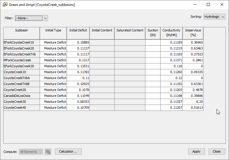
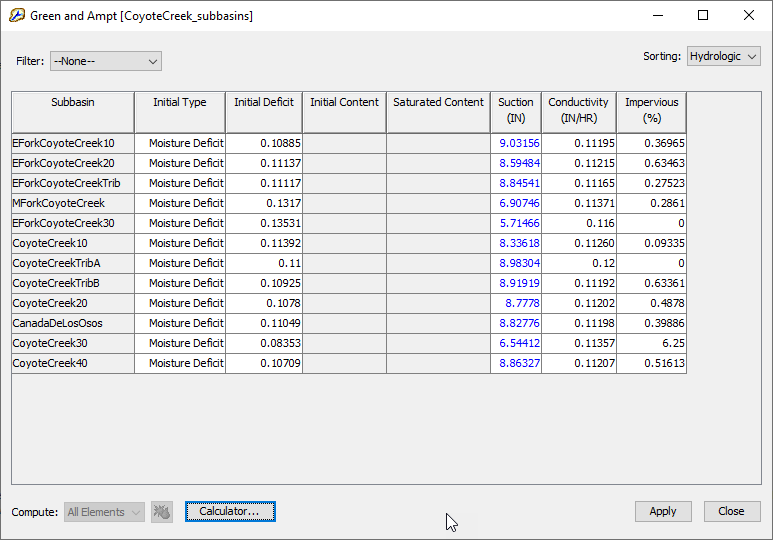
- Select the Parameters→Loss→Green and Ampt menu option to open the Green and Ampt global editor as shown below. All parameters except for the wetting front suction have already been estimated.
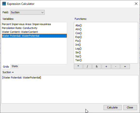
- Click the Calculator... button at the bottom of the global editor. The following figure shows the Expression Calculator. Select the Suction parameter in the upper left. Select the Grids tab in the Variables panel. The grids tab in linked to all parameter grids that have been added to the project (all grids in ASCII and GeoTIFF format). As shown below, the equation panel shows the equation entered to estimate the subbasin average wetting front suction. The water potential grid is referenced; therefore, the program will use zonal statistics to compute the average value for each subbasin in the basin model when the Calculate button is pressed.
- The following figure shows the estimated Green and Ampt parameters. Click the Apply and Close buttons.
Select the 1982_subbasins simulation run and compute the simulation. View the results at the FS77 sink element (this is the most downstream point in the model). Notice the computed hydrograph matches the observed hydrograph very well for this event. The other model parameters were modified (initial parameter estimates had been modified to calibrate the model). The saturated hydraulic conductivity was reduced from initial estimates, the R/(R+TC) ratio was modified, and the baseflow parameters were determined through trial and error. 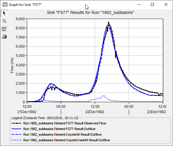
Download the final project files here - Final_ExampleProject.zip