Comparing HEC-HMS Discretization and Transform Options

CoyoteCreek.zip

The purpose of this tutorial is to provide information about discretization and transform methods in HEC-HMS. The example project can be downloaded and opened to walk through information presented below. You must use HEC-HMS version 4.9 to open the project. HEC-RAS 6.0 was used to generate the 2D grid and hydraulic property HDF file. The example project also contains additional precipitation and flow data, for five additional flood events if you are interested in testing and calibrating models to other floods. The 2D Diffusion Wave transform model and simulation were developed following the same procedure shown here - Creating a Simple 2D Flow Model within HEC-HMS.

Introduction

HEC-HMS includes several transform methods. Some methods allow the modeler to enter the unit hydrograph while synthetic unit hydrograph options allow the modeler to enter information about the subbasin response (routing response) and then the program computes the unit hydrograph. There are also additional transform options, the kinematic wave transform option and the ModClark transform method. The ModClark transform method is a quasi-distributed unit hydrograph option where excess precipitation is routed from grid cells within a gridded representation of the subbasin to the subbasin outlet using translation and a linear reservoir. The time component (translation) is based on the travel length for each cell and the time of concentration for the subbasin. The release of HEC-HMS 4.7 provided a new a new subbasin transform method, the 2D Diffusion Wave transform method. The 2D Diffusion Wave transform method is a true cell to cell routing model, it is the same routing model (code) in HEC-RAS.

The release of the new 2D transform method in HEC-HMS also coincides with the requirement for the modeler to define a discretization method for a subbasin element. The selection of the discretization method helps when configuring hydrologic processes and process parameters. Subbasins can be modeled as a lumped area, subdivided into a structured grid (a standard hydrologic grid or a UTM grid), or subdivided into an unstructured mesh.

In addition to breaking a subbasin up into a grid, or mesh, watershed discretization also includes dividing the watershed into smaller subbasins. The GIS delineation tools in HEC-HMS allow modelers to customize the watershed delineation with many smaller subbasins or a few larger subbasins. HEC-HMS is flexible, a modeler can choose only one subbasin to represent the entire watershed or many subbasins and reaches can be used to represent smaller areas within the watershed. The decision about how to discretize a watershed model has implications for the model's development, application, and future use. The level of discretization should be made considering watershed characteristics and the boundary condition data available to calibrate the model. This tutorial shows different discretization and transform methods and how they can be applied to an HEC-HMS application. 

Watershed Description

The area modeled in this tutorial is part of the Coyote Creek watershed in Northern California. The watershed modeled is approximately 109 square miles and is located just south and east of San Jose, CA. The location of the watershed is shown below.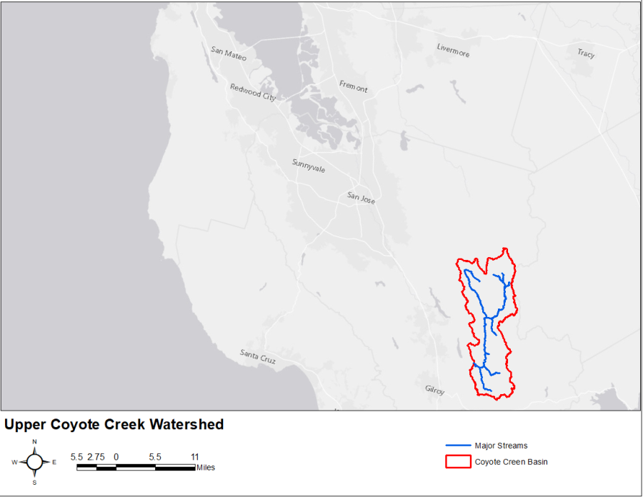

Terrain data was downloaded from the USGS National Map Viewer: https://viewer.nationalmap.gov/basic/. The terrain data was reprojected and the vertical units were converted to feet. Published streams from the National Hydrograph Dataset (NHD) were burned into the terrain as well. The terrain data was used to delineate subbasin and stream elements within HEC-HMS. The terrain data was also used by the HEC-RAS 2D preprocessor to extract hydraulic properties for each cell and cell face in the 400-ft unstructured mesh. The following figure shows the watershed on top of an aerial image; notice the watershed is in the coastal mountains.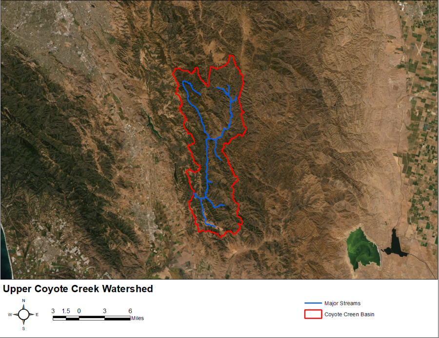  

Landuse data was gathered from the National Land Cover Database (NLCD) 2016. As shown below, land uses within the watershed are mixed forest, grassland, and shrub/scrub. Soil data from the SSURGO database was used to create raster datasets of soil properties, like saturated hydraulic conductivity. The soil property datasets were used to estimate Green and Ampt parameters.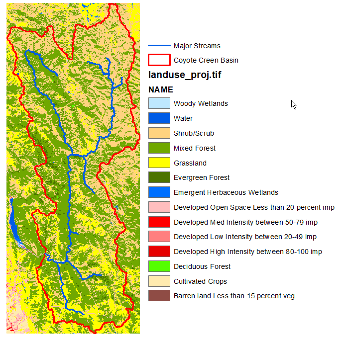

Precipitation and flow information were provided by staff at the California Department of Water Resources. Both the precipitation and flow data were recorded at 15-minute intervals. The follow figure shows the precipitation gage locations. The flow gage is located at the outlet of the watershed area. HEC-GageInterp was used to interpolate the point rain gage data to create precipitation grid sets for six storm events (a 2000-meter grid spacing was used for the interpolation). The PRISM 30-year average precipitation dataset was used as a bias grid in the interpolation process.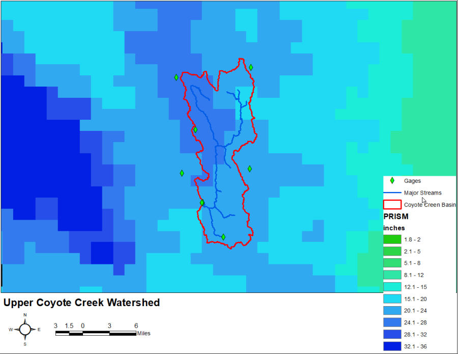

Different Discretization Options in HEC-HMS

The discretization method describes how precipitation losses and excess are computed and then how the excess precipitation is transformed to surface runoff. There three subbasin discretization methods in HEC-HMS are none, structured grid, and unstructured mesh.

A discretization of none means all processes are averaged for the subbasin and only unit hydrograph and kinematic wave transform methods can be used. Even when subbasin average modeling is applied, the level at which subbasins are delineated is part of the discretization process. As shown below, the Coyote Creek model was sub-delineated into twelve subbasins. Instead of averaging precipitation, losses, and performing routing for the entire watershed, computations are performed for each subbasin, combined, and then routed in the stream network. Sub-delineating subbasin elements allows the modeler to take advantage of spatial precipitation information, and more accurately model heterogeneous conditions in the watershed. In addition, breaking the model up into subbasin element provides a way to get information within interior locations in the model domain. Treating the area as one lumped watershed means results are only available at the outlet. Treating the model as twelve subbasins means there is simulated flow information at multiple locations within the watershed.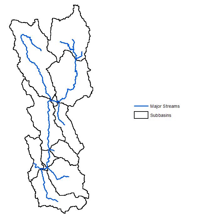

The structured grid discretization method breaks the subbasin into uniform grid cells using either the Standard Hydrologic Grid (SHG) or UTM Grid projections. The modeler can choose the grid cell size for both grid projections. A 2000-meter SHG is shown on top of the Coyote Creek watershed below. The structure grid option can be used with gridded or lumped (basin averaged) loss methods and with unit hydrograph and the ModClark transform methods. When lumped loss and unit hydrograph methods are used (excluding ModClark), gridded precipitation is converted to basin average precipitation. Gridded or non-gridded precipitation can be used with a structured grid.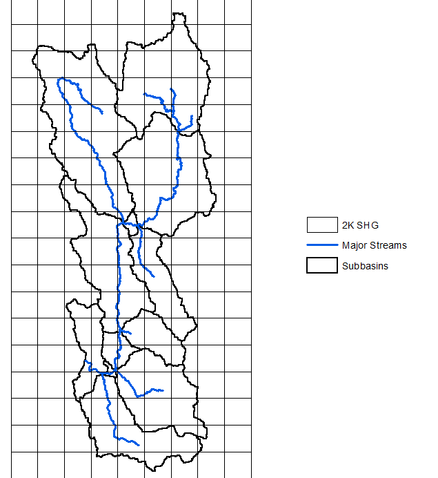

The unstructured discretization method is used to create a 2D mesh that can be used with the 2D Diffusion Wave transform method. Currently, the modeler must create the 2D mesh and compute the mesh properties in HEC-RAS before referencing the mesh in HEC-HMS. A portion of a 400-ft unstructured mesh is shown on top of the Coyote Creek watershed. The unstructured mesh option can be used with gridded or lumped loss methods and with unit hydrograph, ModClark, and 2D Diffusion Wave transform methods. Gridded or non-gridded precipitation can be used with an unstructured mesh.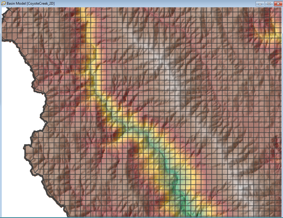

The File-Specified discretization option allows the modeler to choose different file types that represent a structured or unstructured discretization. The file types include *.mod, *.sqlite, *.hdf5 and *.hdf files. The *.mod file is the old HEC-GeoHMS file type for a structured grid. HEC-HMS creates *.sqlite files to save structure grid information when the structured grid is computed within HEC-HMS. The *.mod is being phased out as the *.sqlite file format is the preferred option for structured grids (the *.sqlite file contains geometric information whereas the *.mod file simply identifies which grid cells are located in each subbasin). Refer to this tutorial for information about how to quickly create a structured grid for an old project that might have no geospatial information - Applying Gridded Precipitation to a Non-Georeferenced Project - Structured Discretization. The *.HDF and *.HDF5 file formats are used to store the unstructured mesh information.

Different Transform Options in HEC-HMS

The unit hydrograph methods in HEC-HMS have been applied to a wide range of subbasin sizes and to many types of studies (forecasting, floodplain mapping, planning, dam and levee safety, and others). The 2D Diffusion Wave transform option provides a new way to model hydrologic processes in a watershed. The scale of the hydrologic processes becomes smaller when breaking a subbasin up into smaller units (an unstructured mesh) and routing excess precipitation across the land surface. Unit hydrograph methods provide routed flow at the outlet of the subbasins. Flow at interior locations is not known with the unit hydrograph method unless the subbasin is broken up into smaller subbasins. The 2D Diffusion Wave transform method does allow modelers to see how flow varies across the subbasins/mesh. Also, the 2D Diffusion Wave transform method does not have the same inherent assumptions that are part of the unit hydrograph approach. The two main assumptions with the unit hydrograph approach are the assumptions of linearity and time-invariance.

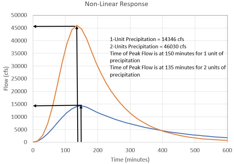
Linearity in the unit hydrograph applications means that 2 units of excess precipitation will result in a hydrograph that is 2 times larger than a hydrograph with 1 unit of excess precipitation. There is no adjustment to the time or shape of the unit hydrograph as the precipitation intensity changes. Due to the linearity assumption, it is important to calibrate the model to similar magnitude events used for model prediction.

The following figures illustrate the linear assumption. The first figure shows a hydrograph generated by 1 unit of precipitation. Using a linear assumption about runoff response, 2 units of precipitation generate hydrograph ordinates that are 2 times larger than the 1 unit hydrograph. The peak flow is doubled, but the time of peak flow does not change. The second figure shows a non-linear response where the hydrograph from 2 units of precipitation is more than three time larger than the peak flow from 1 unit of precipitation and the peak flow occurs 15 minutes earlier.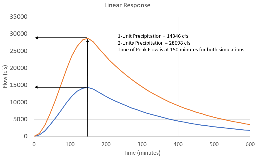

The time-invariance assumption means the unit response does not change in time; the watershed will respond the same for the case where there was one unit of precipitation directly followed by another unit of precipitation vs. the case where there was a considerable amount of time separating the units of precipitation. It is expected that the case where 1 unit of precipitation directly following precipitation will have a larger peak flow and shorter time to peak flow due to excess precipitation from the preceding rainfall already in the channel network. Additional precipitation while water is in the channel network will result in faster water velocities and an overall different hydrologic response.

The following figure shows results from two scenarios (the scenarios were modeled with the 2D Diffusion Wave transform method in HEC-HMS). The smaller runoff hydrograph was generated by one unit of precipitation that fell on a dry watershed. The larger runoff hydrograph was generated by one unit of precipitation that fell six hours after an event that also included 1 unit of precipitation. Notice the baseflow is much higher for the scenario with an antecedent event. There was still water from the antecedent event moving across the watershed when the second event occurred. This example shows that the antecedent event resulted in a shift of 30 minutes for the time of peak flow and the antecedent event amplified the magnitude of peak flow.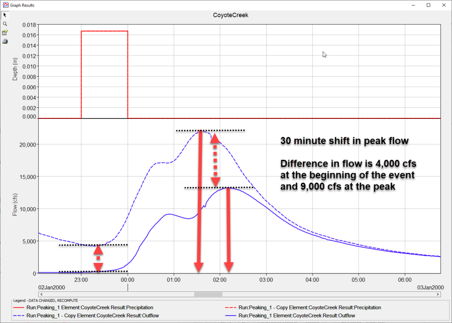

Application of Different Discretization and Transform Options to the Coyote Creek Model

The HEC-HMS model linked to this tutorial has five basin models and five corresponding simulation runs. The subbasin average Green and Ampt loss method was used in all basin models (no gridded loss methods were used). As shown in the table below, the basin models use the ModClark, Clark, and 2D Diffusion Wave transform methods. The linear reservoir baseflow method was used in all basin models. Loss, transform, and baseflow method parameters were adjusted in some of the basin models when calibrating the model to a flood event on December 22, 1982.

Compare Model Results

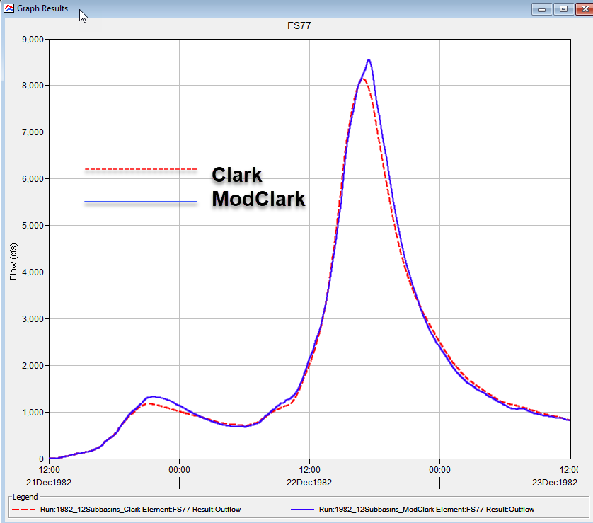
The following two figures show results from the 1982_12Subbasins_ModClark and 1982_12Subbasins_Clark simulations for the December 1982 event. Both models used 12 subbasins to represent the watershed and gridded precipitation. The only difference was the 12Subbasins_Modclark basin model used the ModClark transform method. The 12Subbasins _Clark basin model used the Clark transform method; therefore, the gridded precipitation was converted to basin average precipitation before losses and transform were computed.

Notice how the hydrographs are generally the same in the second figure below. Similar results indicate discretizing the watershed to 12 subbasins captured the spatial variability from the 7 precipitation gages within and around the watershed. Also, further discretizing the precipitation to a 2000-meter grid do not provide much difference in results for this watershed and event.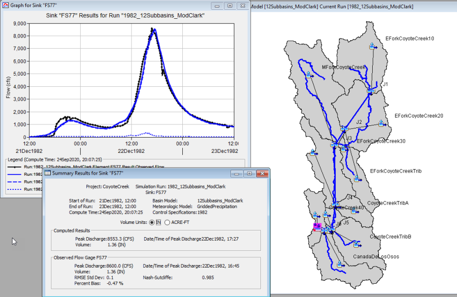


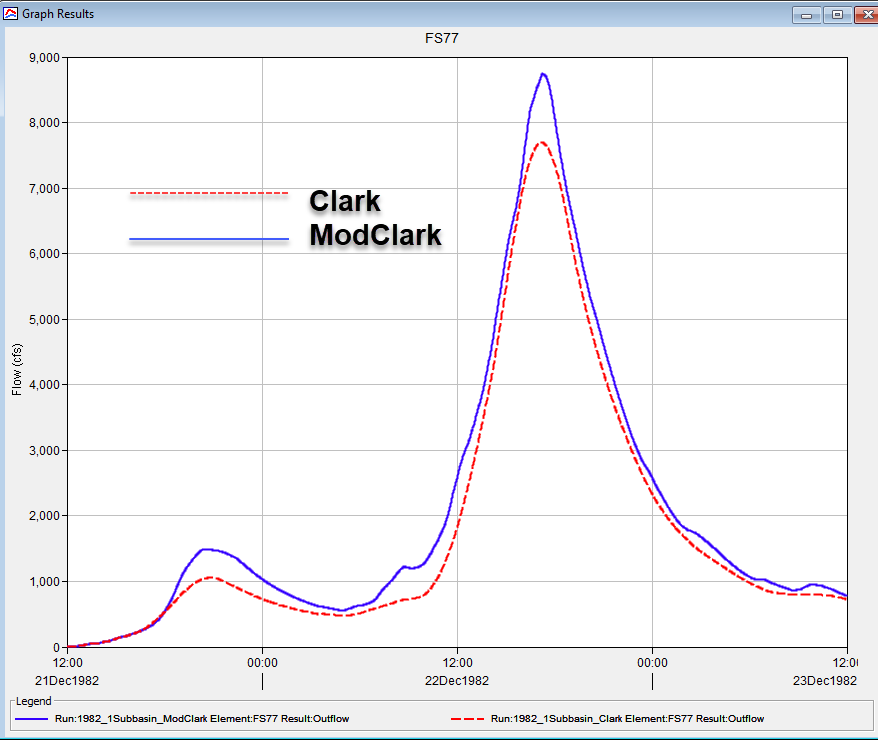
The following two figures show results from the 1982_1Subbasin_ModClark and 1982_1Subbasin_Clark simulations for the December 1982 event. Both models used one subbasin to represent the watershed. The 1Subbasin_ModClark basin model used the ModClark transform method and gridded precipitation. The 1Subbasin_Clark basin model used the Clark transform method, which resulted in the gridded precipitation being transformed to basin average before being applied to the loss computations.

Notice the difference in the simulated hydrographs in the second figure below. Unlike the 12 subbasin model, discretizing the watershed with only one subbasin resulted in much more difference in the gridded (ModClark) and non-gridded (Clark) simulations. The Clark basin model does not take advantage of the spatial variation in the 7 precipitation gages. Even though the 1Subbasin_ModClark basin model only has one subbasin representing the entire watershed, use of the ModClark transform method means HEC-HMS will perform precipitation loss and excess calculations for each of the 106 SHG 2000-meter grid cells in the subbasin before routing excess precipitation to the outlet using the grid cell's time of concentration and the storage coefficient.

The approach followed is for illustrative purposes only. The CoyoteCreek_1Subbasin_Clark basin model could have been calibrated for the 1982 event (the Green and Ampt parameters would be modified). However, this exercise illustrates the need to re-calibrate the model when changing the model structure.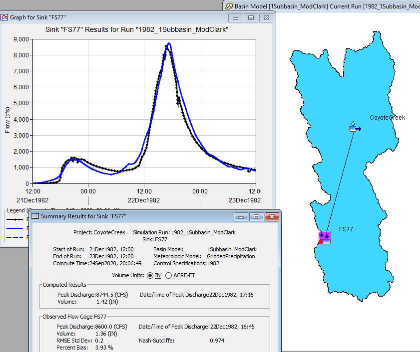


The following figure shows results from the 1982_2D simulation. Gridded precipitation was applied to a 400-ft unstructured mesh. Green and Ampt infiltration was used to model loss and excess for each cell in the mesh. Infiltrated water was routed to the outlet using the linear reservoir baseflow method. The 2D Diffusion Wave transform method was used to route excess precipitation from grid cell to grid cell. The surface roughness values were adjusted to improve timing of the peak flow rates and the Green and Ampt saturated hydraulic conductivity was adjusted to improve runoff volume.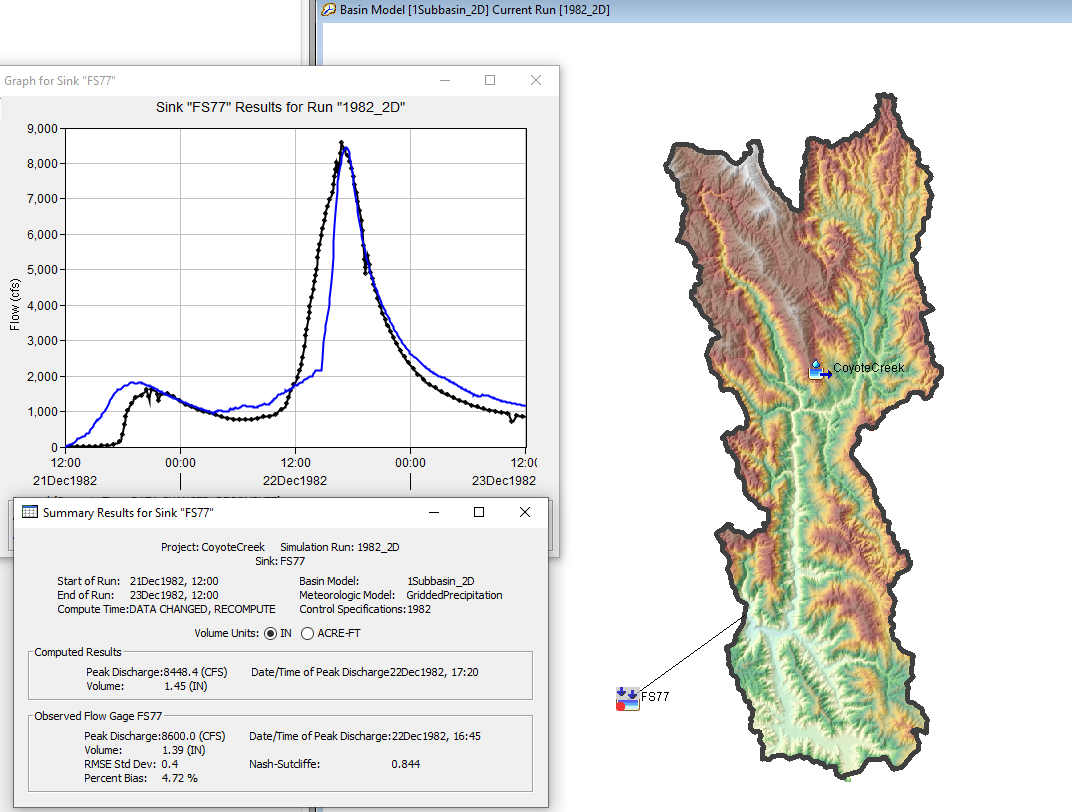

Considerations for Basin Model Discretization and Selection of Transform Methods

Among the many important considerations when choosing how to discretize an HEC-HMS model is the simulation run time. The following table documents the simulation run time for the five simulations in the example project. The 1Subbasin_Clark simulation was the fastest because basin average precipitation was applied to basin average loss, transform, and baseflow methods, and there was only one subbasin. The 1Subbasin_ModClark simulation was just a little longer because gridded precipitation was applied to 106 grid cells within the subbasin. Within each of the 106 SHG 2000-meter cells, loss computations occurred, and then basin average excess was routed using ModClark. The 12Subbasins_ModClark and 12Subbasins_Clark simulations take longer because the basin model was discretized from 1 subbasin to 12 subbasins. Channel routing takes additional time along with modeling hydrologic processed within the 12 subbasins.

The 2D Diffusion Wave transform simulation takes the longest. There are 18,512 cells within the unstructured mesh. The program must compute precipitation for each cell by intersecting it with the gridded precipitation records. Then, losses are computed on each cell before the 2D Diffusion Wave routing was performed.

An important consideration when discretizing a model is the availability of boundary condition data to drive the model. As we saw in the 1Subbasin simulations, using gridded precipitation interpolated from 7 rain gages vs. an area average precipitation time-series for the entire watershed does result in differences in the computed flow. The timescale of the boundary condition data is also important. The precipitation data used for this example was recorded at 15-minute intervals. Subdividing a model into smaller subbasins and/or using the 2D Diffusion Wave transform method should coincide with use of the most detailed precipitation data as possible, in both time and space scales. Using coarse boundary condition data will likely result in unwanted parameter adjustments that are needed to compensate for the quality of the precipitation data. Consider putting more effort into gathering boundary condition data as the level of complexity of the model increases.

The physical characteristics of the watershed should also be considered when discretizing subbasin elements and choosing a transform method. When defining subbasins, an important consideration is whether averaging information across the area appropriate. Large changes in the watershed/stream slope might require delineation of smaller subbasins. Use of the 2D Diffusion Wave transform method requires a different mindset than using unit hydrograph methods. When using the 2D Diffusion Wave method, the watershed does not have to be subdivided into smaller subbasin. One 2D subbasin can be used because physical characteristics of the watershed are accounted for in the 2D mesh properties, and gridded loss parameters can be used as well.

The intended application of the model is an important consideration for selecting discretization and transform methods. Any application that requires an uncertainty or sensitivity analysis where many, many simulations are computed will have to factor in simulation run times. In this case, the 2D Diffusion Wave might not be the best approach, but the 2D Diffusion Wave method could be used to formulate variable Clark TC and R parameters (HEC-HMS includes a variable Clark method where a relationship between time of concentration and the storage coefficient are made with excess precipitation intensity). In some cases, the model will be applied to hypothetical events where the precipitation magnitude exceeds the magnitude of event used for model calibration. The linearity assumption with the unit hydrograph approach illustrates the challenge with applying a model using unit hydrographs to flood simulations larger than the calibration events. In this case, the 2D Diffusion Wave transform method might be the better choice since the physics of surface flow are being modeled; which should account for changes in the runoff response with larger precipitation rates. However, it is noted that the roughness coefficients would not be calibrated for events larger than those used for model calibration.

Finally, where information is needed within the watershed is another important consideration when discretizing a model. In the case of the Coyote Creek application, if flow information is only needed at the outlet of the watershed then a simple representation with only one subbasin element provides the necessary information. The watershed in this example is large enough that spatial precipitation and use of the ModClark transform method could improve the model. Subdividing the model into smaller subbasins provides additional flow values within the watershed; however, additional effort is required to calibrate the model due to additional elements. The 2D Diffusion Wave transform method provides surface flow results and depths throughout the entire subbasin/unstructured mesh.