Download PDF
Download page Task 4: Creating an observed SWE time-series.
Task 4: Creating an observed SWE time-series
Return to Task 3: Normalizing Precipitation Data
Last Modified: 2026-06-24 17:55:14.661

HEC-HMS version 4.14-beta.2 was used to create this example. You can open the example project with HEC-HMS v4.14-beta.2 or a newer version.

The task is part of the Downloading, Importing, and Processing Gridded Data tutorial. You cannot continue with project files from Task 3: Normalizing Precipitation Data. Download new project files here:

Introduction
In this workshop you will use the HEC-HMS Gridded Data Import Wizard to import gridded SWE data. Then you will use the Grid-to-Point utility to create a daily average SWE time-series. Finally you will link the SWE data in HEC-HMS as an observed SWE time-series.
Download University of Arizona SWE data
There are two common sources of Snow Water Equivalent (SWE) data distributed with coverage for the conterminous United States: Snow Data Assimilation System (SNODAS) and University of Arizona (UA). Both provide a spatial SWE product and both are frequently applied as "observed" SWE in HEC-HMS, although both derive SWE by modeling the snow pack with observed inputs from meteorologic inputs, e.g. precipitation and temperature, in a similar manner to the snow pack modeling methods in HEC-HMS.
Download University of Arizona SWE data. The following link is an FTP site with NetCDF files: https://climate.arizona.edu/data/UA_SWE/
Download the UA_SWE_Depth_WY2017.nc file.
Import UA SWE data
Make sure to have the newly downloaded HMS project file open (see top of this page for the download file).
Convert the data in NetCDF format to HEC-DSS using the Gridded Data Import Wizard.
In HEC-HMS File | Import | Gridded Data | Importer to launch the Gridded Data Import Wizard.
On the first step of the wizard select the UA_SWE_Depth_WY2017.nc file.
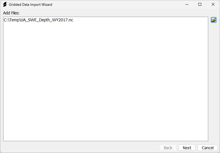
On the second step of the wizard select the "SWE" variable for import.
On the third step of the wizard specify resampling parameters:
- The Clipping datasource specifies the extent to which the data will be clipped to. Use the shapefile that was exported in Exporting a clipping shapefile.
- The Target WKT is the projection, in Well Known Text format, that the data will be projected to. Use the globe on the right to select the SHG projection.
- The Target cell size is the grid cell size that the data will be resampled to. Use the grid button on the right to select 2000 meters.
- The Resampling method is the method used to resample the data. Select the Bilinear resampling method.

On the fourth step of the wizard save the data to a file named UA_SWE.dss.
Click Next to import that data.

You will get a warning about NetCDF files not containing "time_bnds" variable. UA SWE data currently has this issue. See Vortex documentation for more information. This means there is not enough information to read the time step of the data, and the values are read as instantaneous. We will proceed with the instantaneous assumption for this workshop. However, this assumption may have implications depending on data type and application.

Convert UA SWE data to a time-series
In HEC-HMS, from Tools | Data | Grid-to-Point, launch the Grid-to-Point Wizard.
In the first step of the wizard select the UA_SWE.dss file. Select all gridded records.
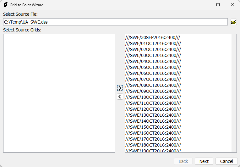
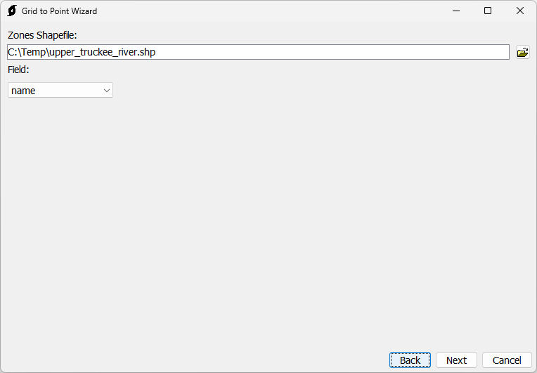
In the second step of the wizard, specify zonal statistics parameters:
- The Zones shapefile defines the geometries for which the zonal statistics will be calculated. Select the shapefile that was created in Export a clipping shapefile.
- The Field is the basis for the HEC-DSS pathname B-part for the HEC-DSS record that will be created. Select the name field.
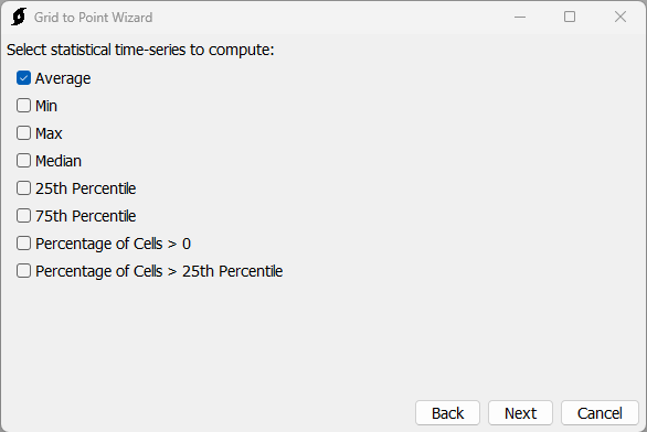
On the third step of the wizard, select Average.
On the fourth step of the wizard, write the time-series to the file <path to>/Upper_Truckee_River/data/Obs_Data.dss.
If prompted to overwrite, select "Yes". You will not be overwriting the HEC-DSS file, but appending it.
Set the F-part for the written record to "UA SWE".
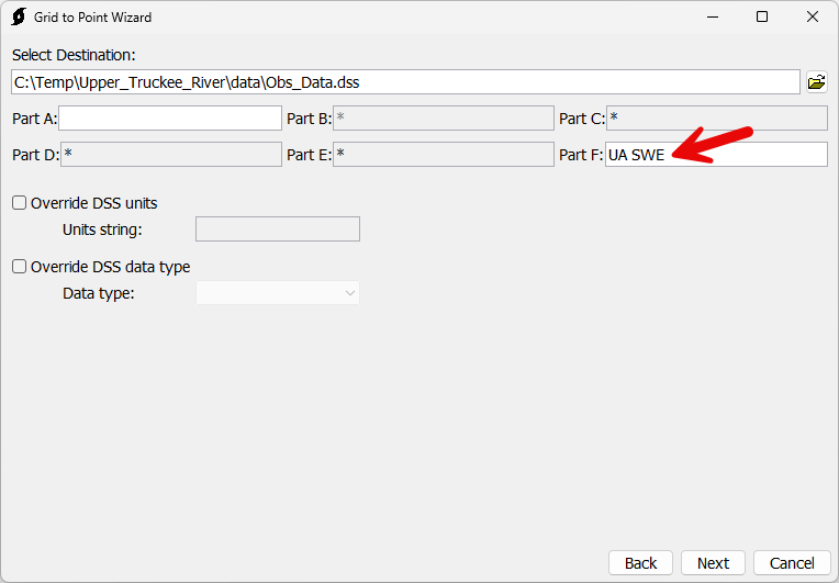
Click Next to proceed with the zonal statistics calculation.
Apply the SWE time-series as an Observed SWE time-series in HEC-HMS
Create a new SWE time series gage.
From Components | Create Component | Time-Series Data launch the Create A New Time-Series Data dialog.
Set the time-series data Name to UpTruckeeRv_S10_UA.
Set the Data Type to Snow Water Equivalent Gages.
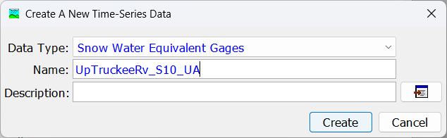
In the Component Editor for the UpTruckeeRv_S10_UA time-series data data, set DSS Filename to <path to>/Upper_Truckee_River/data/Obs_Data.dss. Set the DSS Pathname to //UPTRUCKEERV_S10/SWE/01JAN2016 - 01JAN2017/1DAY/UA SWE/.

In the WY2017_TI_UA basin model component editor, Options tab, set the Observed SWE to UpTruckeeRv_S10_UA.
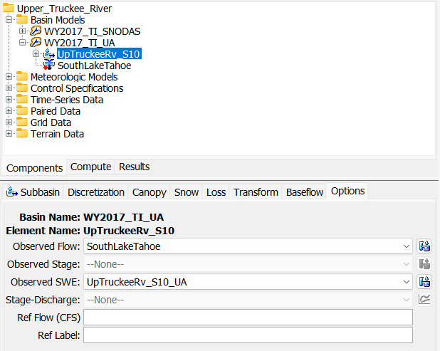
Run the WY2017_MRMS_UA simulation run.
Compare Observed SWE time-series from the WY2017_MRMS_UA and WY2017_MRMS_SNODAS simulations.

Notice the SNODAS and UA SWE have discrepancies but trend similar. It is important to remember these are modeled products and are not observations.
Summary
In this tutorial:
- University of Arizona SWE data was downloaded,
- the Gridded Data Import Wizard was used to import SWE data to HEC-DSS,
- the Grid-to-Point utility was used to extract a daily SWE time-series,
- and the daily SWE time-series was applied as an Observed time-series in HEC-HMS.
You can download final project files for this task here:
This concludes the Downloading, Importing, and Processing Gridded Data tutorial.